
Start / Quick start
Quick start
This page takes you from two arrays, a measured value and its error for each object,
to a population with its uncertainty. It needs binference with the plot extra
(Install). If your data are posteriors, samples, counts or classifier outputs,
Is binference right for my data? names the constructor to use instead.
Your data
Here a simulation stands in for your data: 2000 galaxies with photometric redshifts
z_obs: distances estimated from each galaxy’s colours. Their Gaussian errors z_err
lie between 0.05 and 0.2. Choose bins that cover the range of the true values: here 15
bins of width 0.2 on \([0, 3]\). Replace the simulation with your own arrays.
import binference

bins = binference.Bins.linear(0.0, 3.0, 15)
mock = binference.simulate.mock_1d(2000, bins, rng=42)
z_obs, z_err = mock.measurements["mean"], mock.measurements["sigma"]
Likelihoods
from_gaussian turns each measurement into a bin-averaged likelihood: the
probability of the measurement if the true value lay in each bin.
lk = binference.Likelihoods.from_gaussian(z_obs, z_err, bins)
lk
Likelihoods(N=2000, K=15, dense, bins=Bins(K=15, range=(0, 3)))
Infer the population
One call infers the population fractions \(\rho\). The default engine,
method="auto", chooses an exact sampler and records why.
result = binference.infer(lk, rng=1)
result.info["auto_reason"]
'conjugate prior, missing information 0.92'
infer checks convergence after the fit and warns if the chains disagree or give too
few effective draws. No warning appeared here.
Read the summary
result.summary()
binference fractions posterior (gibbs, 13536 draws; inputs: gaussian)
       bin       mean         sd     median        q16        q84   ess_bulk   rhat  support
  [0, 0.2)    0.01408   0.004688     0.0137   0.009408    0.01874       2038  1.001    80.32
[0.2, 0.4)    0.07883    0.01149    0.07864    0.06743    0.09029       1509  1.002    161.9
[0.4, 0.6)     0.1508    0.01569     0.1507     0.1351     0.1664       1073  1.004    231.5
[0.6, 0.8)     0.1174    0.01615     0.1172     0.1013     0.1337      799.3  1.006    234.5
  [0.8, 1)      0.103    0.01526     0.1031    0.08752     0.1182        924  1.006    208.6
  [1, 1.2)    0.08355    0.01428    0.08294    0.06942    0.09788      978.5  1.005    191.2
[1.2, 1.4)      0.103    0.01459     0.1029    0.08848     0.1176      985.4  1.003      197
[1.4, 1.6)    0.09893    0.01456    0.09856    0.08464     0.1135      957.5  1.002    203.4
[1.6, 1.8)     0.1158     0.0144     0.1158     0.1015       0.13      976.4  1.002    198.3
  [1.8, 2)    0.08231    0.01258    0.08206    0.06964    0.09467       1059  1.001    153.5
  [2, 2.2)    0.03933   0.008923    0.03921     0.0304    0.04814      816.5  1.002    85.84
[2.2, 2.4)   0.008637   0.004467   0.008247   0.004074    0.01312       1016  1.002    37.24
[2.4, 2.6)   0.002714   0.001902   0.002379  0.0008271    0.00458       1750  1.003    12.52
[2.6, 2.8)   0.001061  0.0009423  0.0008085  0.0002177   0.001918       5005      1    3.724
  [2.8, 3)  0.0005444  0.0005463  0.0003753  9.536e-05  0.0009934  1.187e+04      1   0.5624
The title names the engine, the number of draws and the kind of input. The table has one row per bin:
Column |
Meaning |
|---|---|
|
the bin’s edges |
|
the posterior mean and standard deviation of the bin’s fraction \(\rho_k\) |
|
the posterior median of \(\rho_k\) |
|
the ends of the central 68% credible interval; |
|
the effective sample size: how many independent draws the correlated draws are worth |
|
the split R-hat: close to one when the chains agree |
|
the data support: how many objects’ worth of likelihood falls in the bin |
The Defaults page gives the R-hat and ESS limits that check()
applies. In the last bin, the prior sets the fraction: see data support.
Plot it
import matplotlib.pyplot as plt

fig, ax = plt.subplots()
fig.set_figheight(4.4)
result.plot(ax=ax, truth=mock.truth.rho)
ax.get_legend().set(loc="lower left", bbox_to_anchor=(0, 1))  # above the plot
ax.set_xlabel("z");
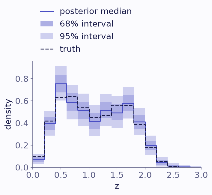
The population inferred from 2000 simulated galaxies: the posterior median density with its 68% and 95% bands, and the true density (dashed).
Your own data have no truth; leave it out.
Use the draws
Every quantity computed from the population has an uncertainty. functional
evaluates a function on each posterior draw, here the mean redshift:
zbar = result.functional(lambda rho: rho @ bins.centers)
print(f"mean redshift: {zbar.mean():.3f} ± {zbar.std():.3f}")
mean redshift: 1.116 ± 0.013
Each galaxy’s posterior under the population, its hierarchical posterior, is narrower than its own likelihood wherever the population is informative. Here is the first galaxy’s, rounded:
result.assignment_probabilities()[0].round(2)
array([0.  , 0.  , 0.  , 0.  , 0.  , 0.  , 0.02, 0.27, 0.58, 0.12, 0.  ,
       0.  , 0.  , 0.  , 0.  ])
Next
Gaussian measurements: a redshift distribution goes further with a similar mock: stacking, correlated bins, smoothness priors and the realised sample.
The results guide lists everything a result holds.
The engines guide explains how
method="auto"chooses.