
Tutorials / Gaussian measurements: a redshift distribution
Gaussian measurements: a redshift distribution
This tutorial infers the redshift distribution of 2000 galaxies. Each galaxy has a photometric redshift with a Gaussian error of its own. The tutorial compares the result with stacking the galaxies’ likelihoods. It then derives quantities with error bars, and shows what the population says about single galaxies.
import matplotlib.pyplot as plt
import numpy as np

import binference
from binference.plotting import SAMPLE_COLOR
A mock catalogue
binference.simulate.mock_1d() draws true redshifts \(z\) from a population with two
peaks. It adds Gaussian errors with standard deviations between 0.05 and 0.2. The 30 bins
on \([0, 3]\) are 0.1 wide, so the errors span half a bin to two bins. The
mock catalogue holds the likelihoods, the truth and the measurements.
mock = binference.simulate.mock_1d(2000, rng=42)
lk, bins = mock.likelihoods, mock.bins
print(lk)
print("measured z of the first galaxies:", mock.measurements["mean"][:4].round(2))
print("their errors:                   ", mock.measurements["sigma"][:4].round(2))
Likelihoods(N=2000, K=30, dense, bins=Bins(K=30, range=(0, 3)))
measured z of the first galaxies: [1.66 0.72 1.74 1.45]
their errors:                    [0.13 0.18 0.09 0.05]
Each galaxy \(i\) contributes one row of bin-averaged likelihoods \(L_{ik}\), one value per bin \(k\). Five of the rows look like this:
fig, ax = plt.subplots()
L = lk.toarray()
for i in range(5):
    ax.step(bins.edges[0], np.append(L[i], L[i, -1]), where="post", color=SAMPLE_COLOR, lw=1.2)
ax.set(xlabel="z", ylabel="likelihood", xlim=(0, 3));
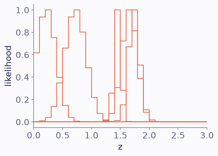
Bin-averaged likelihoods of five galaxies, each scaled to a maximum of one.
Stacking versus the hierarchical posterior
Stacking adds up the galaxies’ likelihoods and gives no error bars. It is the first step of EM, which converges to the most likely population (theory). binference samples the posterior of the population fractions \(\rho_k\) instead, here with NUTS:
stack = lk.stack()
result = binference.infer(lk, rng=1, n_samples=500)   # method="auto" picks the engine
print(result.info["auto_method"], "-", result.info["auto_reason"])
result
nuts - the Laplace importance check failed
PopulationResult(method='nuts', kind='fractions', K=30, n_chains=4, n_draws=2000)
fig, ax = plt.subplots()
result.plot(ax=ax, truth=mock.truth.rho, stack=stack, sample_color=SAMPLE_COLOR, label="median")
ax.legend(ncol=3, loc="lower left", bbox_to_anchor=(0, 1))    # above the plot
ax.set_xlabel("z");
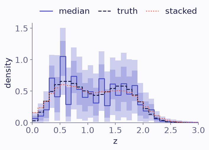
The population posterior under a flat Dirichlet prior, with the truth (dashed) and the stack (dotted). The bands hold 68% and 95% of the posterior.
The bands are wide and the median is jagged. The errors are as wide as the bins, so the data barely tell neighbouring bins apart. Under the flat Dirichlet prior, mass moves freely between those bins, so they are strongly anti-correlated:
corr = result.corr()
print("correlation of bin 10 with bins 9, 10, 11:", corr[10, 9:12].round(2))
correlation of bin 10 with bins 9, 10, 11: [-0.67 1. -0.65]
The summary table gives the numbers per bin and the convergence diagnostics:
result.summary()
binference fractions posterior (nuts, 2000 draws; inputs: gaussian)
       bin       mean         sd     median        q16        q84  ess_bulk    rhat  support
  [0, 0.1)   0.007374   0.003899    0.00705   0.003471    0.01123      1271   1.003    32.63
[0.1, 0.2)    0.01169    0.00817    0.01042   0.003195    0.02035     919.1   1.001    47.69
[0.2, 0.3)    0.02162    0.01305    0.02065   0.007537    0.03516     985.9   1.001    68.66
[0.3, 0.4)    0.06936    0.02167    0.07115    0.04708    0.09091      1251   1.001    92.99
[0.4, 0.5)    0.04469    0.02746    0.04131    0.01648    0.07248      1110   1.003    110.8
[0.5, 0.6)     0.1028     0.0277     0.1052    0.07412       0.13      1412   1.002    121.1
[0.6, 0.7)    0.03298     0.0231    0.02918   0.009643    0.05632      1142   1.001    118.8
[0.7, 0.8)     0.0727    0.02548    0.07366    0.04671    0.09824      1168   1.002    115.5
[0.8, 0.9)    0.05407    0.02528    0.05322    0.02795    0.07964     896.8   1.002    108.6
  [0.9, 1)    0.04103     0.0217    0.04032    0.01772    0.06311     754.8   1.003    99.93
  [1, 1.1)    0.04893    0.02141    0.04939    0.02621    0.07044     859.7   1.004     95.6
[1.1, 1.2)    0.03346    0.02099    0.03152    0.01112    0.05552     994.6   1.007    95.46
[1.2, 1.3)    0.06932     0.0234    0.07011    0.04719    0.09266      1243   1.002    98.47
[1.3, 1.4)    0.03064    0.02184    0.02711   0.007927    0.05314      1034   1.004    98.64
[1.4, 1.5)     0.0609    0.02314    0.06168    0.03703    0.08426     763.3   1.002    101.1
[1.5, 1.6)     0.0458    0.02563    0.04375    0.01822    0.07287     571.6   1.004    102.4
[1.6, 1.7)     0.0609    0.02642    0.06211     0.0329     0.0887     585.6   1.005    101.7
[1.7, 1.8)    0.04693    0.02586    0.04557    0.01929    0.07353     666.8   1.003    96.49
[1.8, 1.9)    0.05854    0.02266    0.05903     0.0344    0.08261     807.1   1.003     85.8
  [1.9, 2)    0.02963    0.01684    0.02868    0.01105    0.04738     845.7       1    67.54
  [2, 2.1)    0.02013    0.01285    0.01863   0.006234    0.03389      1016   1.001    50.13
[2.1, 2.2)    0.02027   0.009072    0.02042    0.01085     0.0295      1289   1.004    35.97
[2.2, 2.3)   0.006619   0.004822   0.005778   0.001802    0.01161      1133   1.006    23.33
[2.3, 2.4)   0.003303   0.002589   0.002716  0.0008135   0.005939      1666  0.9998    13.92
[2.4, 2.5)   0.001974   0.001672   0.001575  0.0004448   0.003403      2319   1.002    7.998
[2.5, 2.6)   0.001483   0.001285   0.001162  0.0003095   0.002681      1206   1.003    4.495
[2.6, 2.7)   0.001129  0.0009589  0.0008874  0.0002746   0.001987      1764       1    2.589
[2.7, 2.8)  0.0006833   0.000666  0.0004716  0.0001218   0.001253      2075       1    1.121
[2.8, 2.9)  0.0005536  0.0005739  0.0003771  8.667e-05   0.001019      1810   1.001   0.4288
  [2.9, 3)  0.0005075   0.000489  0.0003689  9.795e-05  0.0009083      1967   1.002   0.1371
Derived quantities
Sums and averages over bins are much better determined than single bins, because the anti-correlations cancel. Compute a derived quantity on each posterior draw:
centers = bins.centers
zbar = result.functional(lambda rho: rho @ centers)
f_high = result.functional(lambda rho: rho[centers > 1.5].sum())

print(f"mean redshift:   {zbar.mean():.3f} ± {zbar.std():.3f}   (truth {mock.truth.rho @ centers:.3f})")
print(f"fraction z>1.5:  {f_high.mean():.3f} ± {f_high.std():.3f}   (truth {mock.truth.rho[centers > 1.5].sum():.3f})")
print(f"stacked mean z:  {stack @ centers:.3f}  (no error bar)")
mean redshift:   1.119 ± 0.013   (truth 1.110)
fraction z>1.5:  0.298 ± 0.017   (truth 0.296)
stacked mean z:  1.116  (no error bar)
Adding the per-bin variances ignores the correlations, and gives a much larger error bar on the mean redshift:
naive = np.sqrt(np.sum((result.std * centers) ** 2))
print(f"error ignoring correlations: {naive:.3f}   vs   correct: {zbar.std():.3f}")
error ignoring correlations: 0.125 vs correct: 0.013
If you expect the population to be smooth over a few bins, a smoothness prior narrows the bands; Priors and smoothness compares the priors.
Single galaxies
The population also narrows each galaxy’s redshift. Its hierarchical posterior
\(P(k_i=k\mid D)\) combines its own likelihood with the inferred population. It is
narrower than the likelihood wherever the population changes across the likelihood’s
width. assignment_probabilities() returns these posteriors for every galaxy. The
measure of narrowing here is the ratio of the spreads of the two over the bins:
def spread(p):                       # standard deviation of each row over the bin centres
    return np.sqrt(p @ centers**2 - (p @ centers) ** 2)

own = L * bins.volumes
own /= own.sum(axis=1, keepdims=True)
post = result.assignment_probabilities()
ratio = spread(own) / spread(post)
broad = mock.measurements["sigma"] > 0.15           # galaxies with large errors
print(f"median narrowing, galaxies with errors above 0.15: {np.median(ratio[broad]):.2f}")
median narrowing, galaxies with errors above 0.15: 1.06
The effect is modest: the median ratio is 1.06, so the spread shrinks by about 6%. Here is a typical broad galaxy. It is the one closest to the median narrowing whose true redshift lies inside the central 68% of its posterior:
from binference.plotting import plot_individual

cdf = np.cumsum(post, axis=1)
k_true = bins.index(mock.truth.values)

def inside_68(j):                    # the true bin overlaps the central 68% of the posterior
    below = cdf[j, k_true[j] - 1] if k_true[j] > 0 else 0.0
    return below < 0.84 and cdf[j, k_true[j]] > 0.16

candidates = np.flatnonzero(broad)[np.argsort(np.abs(ratio[broad] - np.median(ratio[broad])))]
i = int(next(j for j in candidates if inside_68(j)))
print(f"galaxy {i}: narrowing {ratio[i]:.2f}")

fig, ax = plt.subplots()
plot_individual(result, i, ax=ax, sample_color=SAMPLE_COLOR)
ax.axvline(mock.truth.values[i], color="k", lw=1, ls=":", label="true z")
ax.set_xlabel("z")
ax.legend(loc="lower left", bbox_to_anchor=(0, 1));    # above the plot
galaxy 35: narrowing 1.06
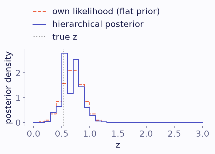
A typical galaxy’s own likelihood (dashed) and its hierarchical posterior (solid). The dotted line marks its true redshift.
The effect grows where the population has sharp features, as in Empirical Bayes deconvolution.
result.sample_values() gives joint draws of the galaxies’ true redshifts.
\(\rho\) describes the population that the galaxies were drawn from; the redshift histogram of these 2000 galaxies, the realised sample, is a different quantity (population versus realised sample).
Next steps
Priors and smoothness compares priors on a sparser catalogue.
Posteriors on a grid and Posterior samples: black-hole masses start from posteriors instead of likelihoods.
Choosing an engine compares the engines.
The guides explain every option.