How it works / Point estimates

Point estimates

How does binference find the single most probable population, and how does it know it has found it? A point estimate maximises the posterior (2) of the model. Three solvers share the work: EM, mix-SQP and L-BFGS. Each estimate carries a certificate of optimality. The answer also depends on the coordinates the posterior is written in, as the last section shows.

EM is iterated stacking

The EM algorithm (Dempster et al. 1977) for (2) with a flat prior is

\[ \rho_k^{(t+1)}=\frac{\hat n_k(\rho^{(t)})}{W} =\frac1W\sum_iw_i\,r_{ik}(\rho^{(t)}). \]

Each step averages the objects’ responsibilities: it stacks the per-object posteriors computed under the current population. Two consequences follow.

• Stacking is one EM step. Stacking posteriors computed under an interim prior \(\pi\) is one EM step started from \(\pi\). It is biased whenever the likelihoods are broader than the features of the population, which is exactly when error bars matter.

• The same iteration recurs across fields. Iterative Bayesian unfolding, Richardson–Lucy deconvolution, EM quantification (Saerens et al. 2002) and the Shepp–Vardi algorithm are all this update. Stopping it early is an implicit regulariser, not a prior.

Conjugate priors keep the update in closed form. A \(\mathrm{Dir}(\alpha)\) prior adds \(\alpha_k-1\) pseudo-counts to \(\hat n_k\) before normalising. With a selection, the expected counts include the missed objects (selection effects). For rates with a \(\mathrm{Gamma}(a_k,b_k)\) prior, the update is \(\lambda_k\leftarrow(\hat n_k+a_k-1)/(S_k+b_k)\). binference accelerates EM with SQUAREM (Varadhan and Roland 2008).

Missing information

EM is slow when the likelihoods are broad. Its speed is set by the missing information, PopulationModel.missing_information:

\[ f=1-\min\operatorname{eig}\left(I_{\rm obs},\,I_c\right). \]

Here \(I_{\rm obs}\) is the observed information in the isometric log-ratios of \(\rho\), and \(I_c\) the information the labels would give if they were known. The smallest generalised eigenvalue picks the direction with the least information relative to known labels. Near that direction each EM step removes only a share \(1-f\) of the remaining error (Dempster et al. 1977).

• \(f\) is near 0 when the likelihoods are narrow compared with the bins, and near 1 when they are broad.

• With a selection, \(I_c\) counts the imputed missed objects too: \(W/(S\cdot\rho)\) objects in all.

• \(f\) is computed on the support of \(\rho\). A fraction at zero is an active constraint, not missing information.

• With include_prior=True, a Dirichlet prior’s pseudo-counts enter \(I_c\) and \(I_{\rm obs}\), as they do in EM.

The same number sets the speed of the Gibbs sampler (Gibbs, explainer V-14) and the choices of auto.

mix-SQP

For Dirichlet concentrations \(\alpha_k\ge1\), the log posterior is concave on the simplex. binference then uses mix-SQP (Kim et al. 2020) instead of EM. Each iteration fits a quadratic model of the objective and minimises it under \(\rho\ge0\), as a non-negative least-squares problem. It converges in tens of iterations however broad the likelihoods are, where EM can need thousands.

A selection makes the likelihood non-concave in \(\rho\). It stays concave in the selected population \(\phi_k=S_k\rho_k/(S\cdot\rho)\):

\[ p(d_i\mid\text{detected},\rho)=\frac{\tilde L_i\cdot\rho}{S\cdot\rho}=\sum_k\frac{\tilde L_{ik}}{S_k}\,\phi_k . \]

The maximum-likelihood estimate does not depend on the coordinates. With the flat prior, binference therefore solves for \(\phi\) and maps back, \(\rho_k\propto\phi_k/S_k\). Other priors do not keep their mode under this change of variables, so they use EM.

Rates with a GammaRates prior of shapes \(a_k\ge1\) reduce to the same problem. Write \(\lambda_k=\Lambda\chi_k/(S_k+b_k)\) with \(\chi\) on the simplex. The total \(\Lambda=W+\sum_k(a_k-1)\) then profiles out. What remains is mix-SQP in \(\chi\), with \(S_k+b_k\) in place of \(S_k\) and a Dirichlet term \(\sum_k(a_k-1)\log\chi_k\).

L-BFGS

The other cases maximise the density in unconstrained coordinates with L-BFGS:

• Priors whose density is unbounded at the edge of the simplex, such as concentrations below one or a Pólya tree. Their mode on the simplex can be exactly zero.

• Priors that are not conjugate, such as the logistic family.

• A selection or response inferred with the population.

MAP lists which solver each case uses. est.info["algorithm"] and est.info["space"] record the choice.

The certificate

At the maximum on the simplex the Karush–Kuhn–Tucker conditions read

\[ g_k=\frac1W\sum_i\frac{w_iL_{ik}}{L_i\cdot\hat\rho}\le1,\quad\text{with equality where }\hat\rho_k>0 . \]

In general, write \(\partial_k\) for \(\partial\log p(\rho\mid D)/\partial\rho_k\) at \(\hat\rho\), including the prior’s and the selection’s terms. binference reports the optimality gap, the KKT gap,

\[ \frac{\max\big(0,\ \max_k\partial_k-\hat\rho\cdot\partial\big)}{\max(W,1)}, \]

for every estimate from EM or mix-SQP (PointEstimate.kkt_gap). With a flat prior and no selection, \(\partial_k=Wg_k\) and \(\hat\rho\cdot\partial=W\), so the gap is \(\max_kg_k-1\). It is infinite where an object has zero likelihood. A fixed point of EM is necessary for optimality but not sufficient; the gap checks the rest.

For rates the conditions are \(\partial\log p/\partial\lambda_k\le0\), with equality where \(\hat\lambda_k>0\). The gap is the larger of \(\max_k S_k^{-1}\,\partial\log p/\partial\lambda_k\) and \(|\lambda\cdot\nabla_\lambda\log p|/(S\cdot\lambda)\), so it does not depend on the units of the exposure.

MAP(tol=) bounds the KKT gap for EM and mix-SQP; for mix-SQP the gap is that of its transformed problem. MAP states the bound for L-BFGS and for runs stopped by round-off.

Two coordinate systems, two modes

The same posterior has a density in each coordinate system. The two densities differ by the Jacobian of the map between the coordinates (coordinates), so they have different modes.

• PopulationModel.log_posterior is the density of the fractions (or rates), without a Jacobian. Its mode is MAP(space="simplex"), which EM and mix-SQP find. Every point estimate reports this density as log_posterior.

• PopulationModel.log_density_unconstrained is the density of \(x\), with the Jacobian. Its mode is MAP(space="unconstrained"). NUTS, Laplace and L-BFGS use it.

log_posterior is NaN for priors without a closed-form density on the simplex, the logistic family. Take a \(\mathrm{Dir}(\alpha)\) prior and objects with known labels, \(n_k\) of them in bin \(k\). The log density on the simplex is then \(\sum_k(\alpha_k+n_k-1)\log\rho_k\), and the unconstrained log density \(\sum_k(\alpha_k+n_k)\log\rho_k\), up to constants. The two modes are proportional to \(\alpha_k+n_k-1\) and to \(\alpha_k+n_k\).

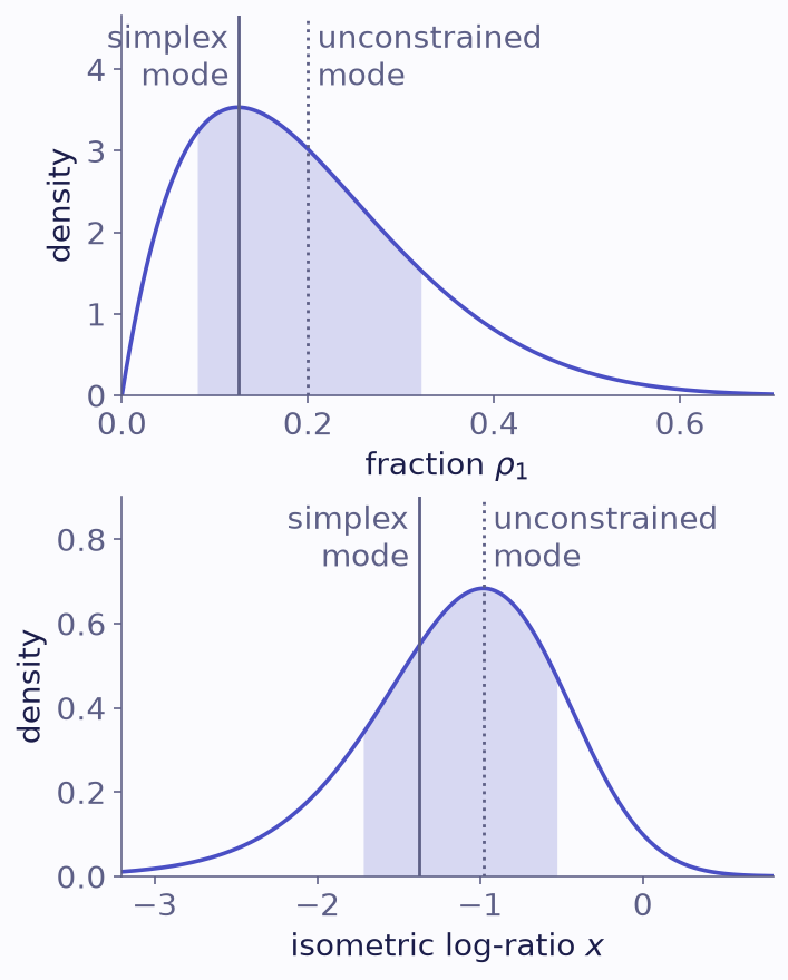
One posterior in two coordinates. Two bins hold one object certainly in bin 1 and seven certainly in bin 2, under a flat prior. The fraction of bin 1 then has a Beta(2, 8) posterior (top), and its isometric log-ratio \(x\) the density below. Each panel’s peak is its own mode. The shaded central 68% interval holds the same draws in both.

Neither mode is “the” answer. The posterior mean and quantiles of any quantity are the same in every coordinate system, because they are properties of the draws. The mode on the simplex can sit on the boundary, with a fraction exactly zero. The unconstrained mode is always interior, which is why the Laplace approximation is centred there (Laplace).