How it works / Engines in detail

Engines in detail

What does each engine compute, and when are its draws exact? Every engine works on the posterior of the model. NUTS and Gibbs draw from it exactly, given enough iterations. Laplace and mean-field VB approximate it, and the bootstrap answers a different, frequentist question. How auto chooses describes how method="auto" chooses between them, and the engines guide how to call them.

NUTS

The No-U-Turn Sampler (Betancourt 2017; Hoffman and Gelman 2014) samples the density of the unconstrained coordinates \(x\) (coordinates). It is exact for every prior, and it is the last candidate of method="auto".

• Trajectories. It uses multinomial sampling along each trajectory and the generalised U-turn criterion, with Stan’s extra checks across merged subtrees.

• Starting points. Chains start at the mode of the unconstrained density, plus Gaussian jitter. Chains can run in parallel processes. They then use the same random streams as a serial run.

• Step size. Dual averaging adapts the step size during warm-up to a target acceptance statistic. The target is higher for logistic priors, whose hyperparameters make the geometry harder (defaults).

• Metric. Warm-up follows Stan’s windows: a fast phase, slow windows that double in length, and a final fast phase. Each slow window estimates the metric from the draws it holds. The metric is diagonal, or dense for logistic priors. The dense metric has a dimension limit in the defaults.

• Curvature. For logistic priors, early in warm-up the engine also starts the metric from the finite-difference curvature \(H\) of the log density. Each later window then shrinks its estimate towards the previous metric. Simplex and rate priors keep Stan’s adaptation unchanged: at single points their curvature is a poor guide to the scales of nearly empty bins.

• Records. Each run records its divergences and the share of iterations that reach the maximum tree depth. It also records the E-BFMI of each chain and the adapted step sizes (validation).

Partial centring

The whitened form of a logistic prior (the logistic family) samples well when the data are weak. With strong data the posteriors of \(s_j(\theta)\) and \(\xi_j\) are strongly and non-linearly correlated. During warm-up NUTS therefore re-parametrises each coefficient \(c_j=s_j\xi_j\) as

\[ c_j=s_j^{\gamma_j}\zeta_j,\qquad\zeta_j\sim\mathcal N\big(0,s_j^{2(1-\gamma_j)}\big). \]

This interpolates between the non-centred form (\(\gamma_j=1\)) and the centred form (\(\gamma_j=0\)). For a Gaussian likelihood with Fisher information \(F_j\), the best choice is \(\gamma_j=1/(1+s_j^2F_j)\) (Gorinova et al. 2020; Papaspiliopoulos et al. 2007). This equals \(1/(-H_{jj})\), with \(H\) the Hessian of the log density in whitened coordinates. NUTS estimates it from finite differences of the gradient at the chains’ positions. The posterior is unchanged; only the coordinates the sampler moves in change.

Centring is safe only where the data determine the scales \(s_j\). Otherwise the centred coordinates have a funnel of their own. With few modes per hyperparameter, such as a handful of bins, the log-fractions \(\eta\) constrain the hyperparameters weakly. NUTS then keeps non-centred (\(\gamma_j=1\)) every mode whose scale depends on an inferred hyperparameter. It does so when the median spread of \(\log s_j\) given \(\eta\) exceeds a limit in the defaults. That spread comes from the curvature of the log density in the hyperparameters at a fixed \(\eta\). info["centring"] holds the weights \(\gamma_j\) used, and results are reported in the non-centred coordinates.

Gibbs sampling

The data-augmentation sampler (Diebolt and Robert 1994; Tanner and Wong 1987) alternates two exact conditional draws of the augmented form:

1. every object’s label, \(k_i\mid\rho\sim\mathrm{Cat}\big(r_i(\rho)\big)\), as vectorised categorical draws;

2. the population given the counts \(n\): \(\rho\mid n\sim\mathrm{Dir}(\alpha+n)\) for a Dirichlet, a Dirichlet per node for a tree, and \(\lambda_k\mid n\sim\mathrm{Gamma}(a_k+n_k,\,b_k+S_k)\) for rates.

With a selection on fractions, each iteration also draws the missed objects from their negative-binomial and multinomial laws (selection effects). A selection inferred from injections adds a third draw, each \(S_k\) from its Beta conditional given the detected and missed counts. An inferred response draws each column from its Dirichlet conditional.

Gibbs needs a conjugate prior and integer weights. Its chains start from draws of the population’s conditional given the expected counts after a few regularised EM steps. With store_labels=True it keeps joint draws of the labels.

Mixing and missing information

Gibbs is exact, but its successive draws are correlated. The correlation grows with the missing information \(f\). In the slowest direction the lag-one autocorrelation is about \(f\), so the integrated autocorrelation time is about

\[ \tau_{\rm int}\approx\frac{1+f}{1-f}. \]

\(f\) rises towards one as the likelihoods widen compared with the bins (explainer V-14).

V-14 · Missing information and Gibbs mixing

likelihood width (bins)

0.30

f = 0.649, so τ ≈ 4.7; lag-one autocorrelation of ρ₇: 0.51

Top: the missing information \(f\) against the width of the likelihoods, in bins, for mock catalogues of 500 objects in ten bins on \([0, 3]\), half of them from two peaks and half uniform, one mock for each width. \(f\) is taken at the mock’s true population, which occupies every bin; the dot marks the chosen width. Bottom: 400 iterations of a Gibbs sampler (data augmentation under the default Dirichlet prior) started at that population, for the bin whose trace has the largest lag-one autocorrelation. The readout gives \(f\), the predicted \(\tau_{\rm int}\approx(1+f)/(1-f)\) and the trace’s lag-one autocorrelation. \(f\) predicts the slowest direction; a single bin mixes somewhat faster.

The figure below shows longer runs, up to likelihoods one bin wide, on a different mock: 1,000 objects in ten bins on \([0,1]\), with \(f\) at the most probable population. Its numbers therefore differ from those of explainer V-14 at the same widths.

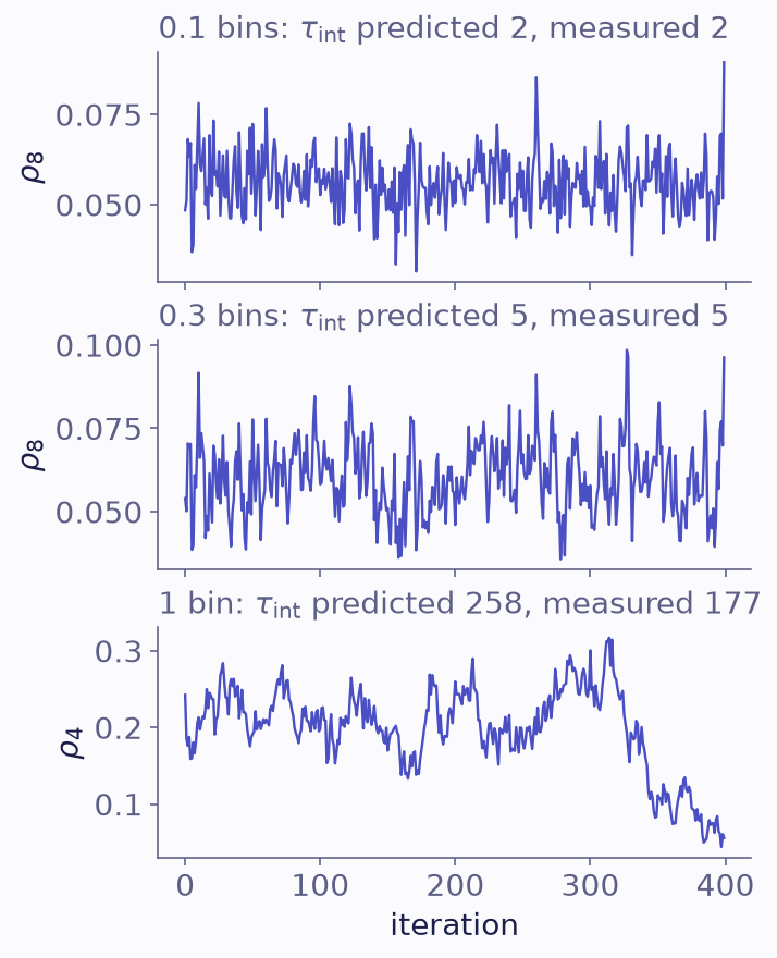
Gibbs traces of the slowest-mixing bin for likelihoods 0.1, 0.3 and 1 bin widths wide, on 1,000 mock objects in ten bins on \([0,1]\): the first 400 of 4,000 iterations of one chain. Each label gives the predicted autocorrelation time \((1+f)/(1-f)\), with \(f\) at the most probable population, and the time measured on all 4,000 iterations. The prediction approximately predicts the slowest direction, not any one bin. A run of about 20 autocorrelation times, as at 1 bin width, underestimates the measured time.

Laplace with importance sampling

The Laplace engine fits a Gaussian in the unconstrained coordinates and corrects it by importance sampling.

1. L-BFGS finds the mode of the unconstrained density. This mode is always interior (two modes).

2. Central differences of the exact gradient give the Hessian \(H\) there. If \(-H\) is not positive definite, its small eigenvalues are raised to a floor (defaults) with a warning.

3. A multivariate Student-\(t\) proposal with covariance \((-H)^{-1}\) draws \(n_{\rm draw}\) proposals, by default a fixed multiple of the draws asked for. Its heavy tails make the correction more robust than a Gaussian proposal.

4. Pareto-smoothed importance sampling (Vehtari et al. 2024) weights the proposals by the exact density, and systematic resampling turns them into draws.

The Pareto shape \(\hat k\) of the weights says whether the correction is reliable. When \(\hat k\) reaches a threshold that depends on \(n_{\rm draw}\) (defaults), the result is flagged approximate and a warning names \(\hat k\). info["ess_importance"] holds the effective number of independent draws among the weighted proposals. In log-ratio coordinates the posterior of a nearly empty bin has a long one-sided tail. The correction therefore often fails with ten or more bins. The Laplace result is then a fast summary of the well-populated bins, not a replacement for NUTS.

Mean-field VB

Mean-field VB (Blei et al. 2017) approximates the posterior of the augmented form by variational factors \(q\), as \(q(\rho)\prod_iq(k_i)\). Coordinate ascent alternates two closed-form updates for a conjugate prior:

\[ q(k_i=k)\propto L_{ik}\exp\mathbb E_q[\log\rho_k], \qquad q(\rho)=\mathrm{Dir}\Big(\alpha+\sum_iw_i\,q(k_i)\Big), \]

with the conjugate update of the other members of the family or of rates in place of the Dirichlet. With a selection, binference sets the expected missed objects from the current mean, a further approximation. Iterations stop when the largest change of the mean falls below a tolerance relative to its largest value.

Factorising the labels from the population ignores exactly the coupling that broad likelihoods create. Mean-field VB’s intervals are therefore too narrow. In a slow test with \(f\) above 0.9, its standard deviations were less than half those of NUTS (validation). Every result is flagged approximate, with a warning.

Bootstrap

The bootstrap refits the most probable population to many resampled catalogues. scheme="nonparametric" resamples objects with replacement, and scheme="bayesian" reweights them with Dirichlet weights (Rubin 1981).

• Integer weights count objects, so a row of weight 5 stands for five objects that are resampled one by one.

• For rates the number of objects is itself random: each object gets a Poisson(1) count or a Gamma(1) weight, so the total varies between replicates.

• Every replicate starts from an interior point. info["n_not_converged"] counts the replicates whose fit did not converge.

The draws are the sampling distribution of an estimator, not a posterior, so the result is flagged approximate. It serves comparisons with frequentist intervals, as in unfolding and empirical Bayes.