Guides / Check a result

Check a result

Check a result in two stages. First, the diagnostics say whether the engine explored the posterior. Second, simulations say whether the posterior is right: whether your likelihoods, prior and engine together give calibrated answers. binference ships the tools for both, the same ones its own test suite uses.

import numpy as np
import binference
from binference import priors
from binference.validation import coverage, exact_posterior, sbc

mock = binference.simulate.mock_1d(800, binference.Bins.linear(0, 3, 15), rng=6)
result = binference.infer(mock.likelihoods, method="nuts", rng=1)

Diagnostics

binference.infer checks every NUTS and Gibbs result and warns about any problem. Call result.check() yourself for other engines, or to change the limits:

d = result.diagnostics                     # rhat, ess_bulk, ess_tail, n_divergent, ...
print(d["rhat"].max().round(3), d["ess_bulk"].min().round(0), d.get("n_divergent"))
problems = result.check()                  # warns, and returns the messages
print(problems)

check() raises a ConvergenceWarning for these problems. The limits are on the defaults page.

• R-hat above its limit: the chains disagree. binference splits each chain in half, so R-hat works for a single chain too.

• Bulk or tail ESS below its limit per chain: too few effective draws. This applies to any Markov chain, including draws wrapped with PopulationResult.from_samples.

• NUTS health: divergent transitions, saturated tree depth, and low E-BFMI.

• Importance weights whose Pareto k-hat is too large, and an optimiser that did not converge.

If the chains disagree or the effective sample sizes are low, run longer. If Gibbs mixes slowly, switch to NUTS. A few isolated divergences among thousands of draws are usually harmless if R-hat and the effective sample sizes pass. Divergences that persist with a higher target_accept mark a region the sampler cannot explore, such as a funnel. Change the prior or its hyperprior rather than ignore them.

A low E-BFMI means that NUTS moves slowly through the energy distribution, so it may under-explore the tails. A longer warm-up or another prior may help; a higher target_accept does not. Otherwise compare the fit with a longer run before you rely on its tails.

Problems with the inputs raise an InputWarning instead. Three are checked:

• the Monte Carlo noise of likelihoods built from samples (Posterior samples);

• binned counts that the response does not describe (Binned measurements and classifiers);

• with check(support_min=...), bins whose data support is low (Choose bins).

Where it can, a warning ends with a hint. After Gibbs, the hint gives the missing information and the autocorrelation time it implies. check(strict=True) raises a binference.DiagnosticsError instead of warning. Every message, its cause and its fix are on the warnings page. A result from an approximate engine has result.approximate set, and its summary says so.

A point estimate has its own check. est.check() warns when the optimiser did not converge, or when the KKT gap per object exceeds kkt_max:

est = binference.infer(mock.likelihoods, method="map")
print(est.check(), est.kkt_gap)

What good and bad look like

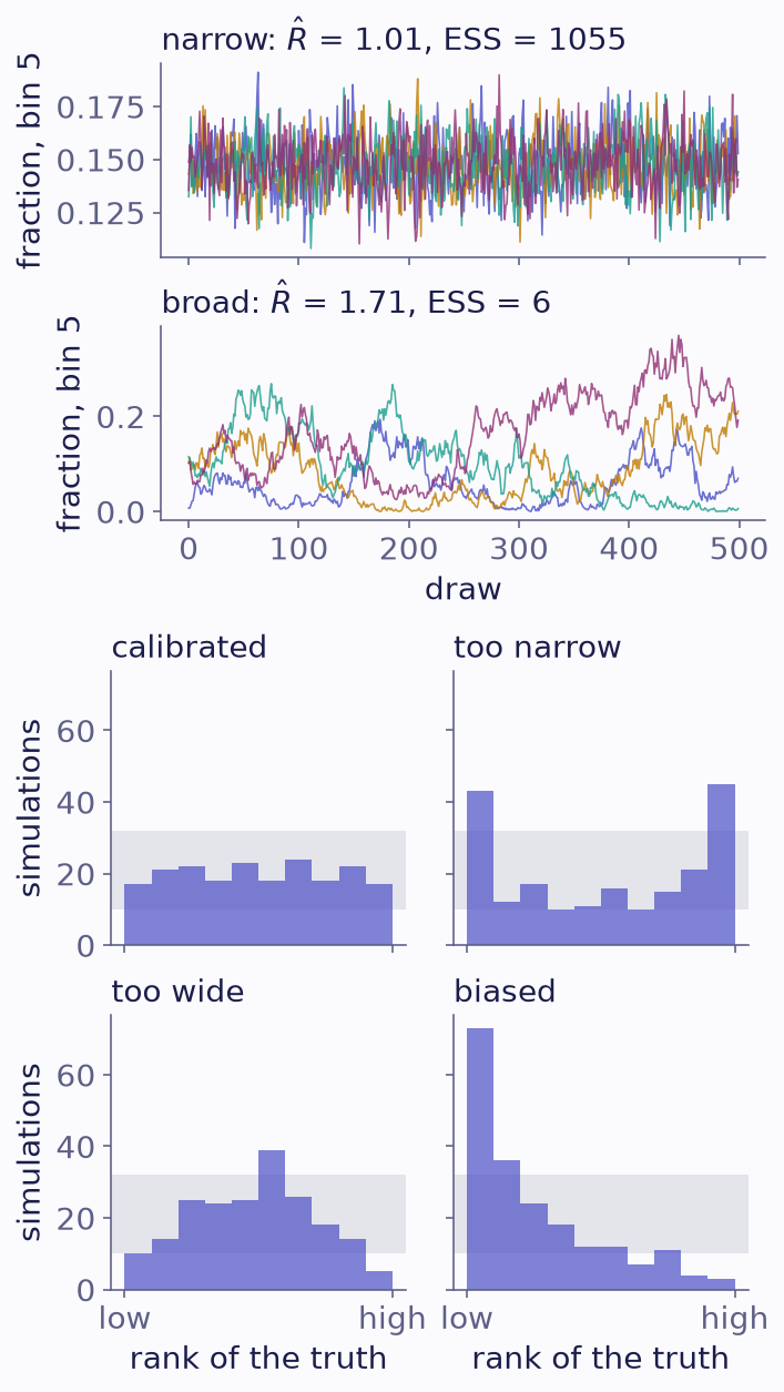
Top: four Gibbs chains for one bin, 1000 objects in ten bins. With narrow likelihoods successive draws are nearly independent. With broad ones the missing information is near one, and the chains have not mixed. Bottom: SBC rank histograms of one bin, from 200 simulations of 100 objects in three bins, fitted by Laplace. The pipelines count each object three times (too narrow), a quarter (too wide), or treat posteriors under a prior favouring the bin as likelihoods (biased). Each bar of a uniform histogram falls inside the grey band 99% of the time.

Traces. Good chains overlap and look like noise around one level. Bad chains wander slowly, or sit at different levels. If they do, run longer or switch engine (Choose an engine).

Rank histograms. SBC ranks the truth among the posterior draws. If the pipeline is calibrated, the ranks are uniform:

• a U shape means the intervals are too narrow;

• a hump means they are too wide;

• a slope means the posterior is biased.

Simulation-based calibration

Simulation-based calibration (SBC; Talts et al. 2018) fits many catalogues simulated from the prior, and ranks the truth among each fit’s draws. How it works is in the theory. Read the rank histograms as in the figure above.

prior = priors.Dirichlet(1.0)
simulate = binference.simulate.prior_predictive(prior, binference.Bins.linear(0, 1, 4),
                                            n_objects=40, noise=0.2)

def fit(lk, rng):
    return binference.infer(lk, prior, method="gibbs", rng=rng, n_chains=4,
                            n_warmup=100, n_samples=600, check=False)

result = sbc(simulate, fit, n_simulations=40, n_draws=19, rng=0)
print(result.names, result.pvalues().round(2), result.passed())
fig = result.plot()

• simulate(rng) returns (likelihoods, true_rho). simulate.prior_predictive builds one from a prior, optionally with a known selection in either mode (selection=, selection_mode=), and you can write your own to include your real selection or noise model. For rate models, return the true rates (as prior_predictive does, drawing the number of objects from a Poisson): ranks and coverage are then computed on the rates.

• fit(likelihoods, rng) returns a result. Use the settings you will use in production.

• log_likelihood. Besides each bin, SBC ranks the joint log-likelihood of the true population. Pass log_likelihood=False to leave it out.

• Tests. result.pvalues() and result.passed() test each quantity’s ranks with a chi-square on their histogram. method="ecdf" uses the ECDF test of Säilynoja et al. (2022) instead. To require both, call result.passed(method="chisquare") and result.passed(method="ecdf").

• Size. A real check needs a few hundred simulations and roughly independent draws: keep n_draws below the effective sample size.

binference’s own slow tests run SBC on its engines and priors (theory).

Coverage

coverage() measures how often central credible intervals contain the truth, for each bin and for any functional. It answers the frequentist question: do my 68% error bars contain the truth 68% of the time?

centers = binference.Bins.linear(0, 1, 4).centers
cov = coverage(simulate, fit, n_simulations=40, levels=(0.68, 0.95),
               functionals={"mean": lambda rho: rho @ centers}, rng=1)
print(cov.levels, cov.average().round(2), cov.stderr().ravel().round(2))

To see how the intervals behave for one particular truth, simulate from a fixed population instead of from the prior (why).

Exact posteriors for small problems

With two or three bins, exact_posterior() gives the exact posterior. Compare any engine against it:

bins = binference.Bins([0.0, 1.0, 2.0, 3.0])
mock = binference.simulate.mock_1d(200, bins, density=np.array([0.5, 0.3, 0.2]), noise=(0.3, 0.8), rng=8)
exact = exact_posterior(mock.likelihoods, priors.Dirichlet(1.0))
res = binference.infer(mock.likelihoods, rng=1, n_samples=1000, n_warmup=500)
print(exact.mean.round(4), res.mean.round(4))
print(exact.std.round(4), res.std.round(4))

Mock catalogues

binference.simulate makes catalogues with known truth for every input type, and prior_predictive makes the simulators that SBC and coverage need.