Guides / Selection and rates

Selection and rates

Real catalogues are incomplete. If the chance of entering the catalogue depends on the quantity you bin, the observed objects are a biased sample of the population. Ignoring that biases the fractions \(\rho\). binference corrects for it, given a selection function: \(S_k\), the probability that an object whose true value lies in bin \(k\) is observed. The same correction gives the total number of objects, including those the catalogue missed.

import numpy as np
import binference

bins = binference.Bins([0.0, 1.0, 2.0, 3.0])
S = np.array([0.9, 0.5, 0.25])                 # detection probability per true bin
mock = binference.simulate.mock_1d(
    3000, bins, density=np.array([0.4, 0.35, 0.25]), noise=(0.3, 0.8), selection=S, rng=7
)
lk = mock.likelihoods.with_selection(None)     # the bare likelihoods
print(mock.truth.rho, mock.truth.n_drawn, "objects drawn,", lk.N, "selected")

Say how the selection acts

The likelihood depends on what the selection acts on, so binference requires you to say which: the selection mode.

selection_mode="on_measurement"

Objects are selected on their measured data: a flux limit on measured fluxes, or a signal-to-noise cut. Here \(S_k\) is the probability that an object in bin \(k\) passes the cut, averaged over its possible data. This mode also covers likelihoods that already include the detection probability, such as a response with its efficiencies.

selection_mode="on_truth"

Objects are selected with a probability that depends on their true value, whatever the measurement noise. Examples are a completeness that depends on true planet radius, or a targeting rate per true class.

Selection.combined(on_truth=..., on_measurement=...)

Both at once: \(P(\text{observed}\mid z,d)=S^{\rm truth}(z)\,S^{\rm meas}(d)\), for example a completeness in redshift together with a magnitude limit.

How each mode enters the likelihood is in the theory.

The mock above selects on the true bin:

right = binference.infer(lk, method="map", selection=S, selection_mode="on_truth").rho
wrong = binference.infer(lk, method="map", selection=S, selection_mode="on_measurement").rho
ignored = binference.infer(lk, method="map").rho
print("truth         ", mock.truth.rho)
print("on_truth      ", right.round(3))
print("on_measurement", wrong.round(3))
print("ignored       ", ignored.round(3))

Ignoring the selection over-weights the well-detected bins. Choosing the wrong mode also biases the fractions. That is why an array passed as selection must come with selection_mode: there is no safe default.

Where to attach it

These three are equivalent:

sel = binference.Selection(S, "on_truth")
a = binference.infer(lk, method="map", selection=sel).rho
b = binference.infer(lk.with_selection(S, "on_truth"), method="map").rho     # on the data
c = binference.PopulationModel(lk, selection=S, selection_mode="on_truth")    # on the model
print(np.allclose(a, b), c)

The simulators and from_binned attach the right selection themselves. simulate.mock_1d(..., selection=S) selects on the truth, and measured_range=(lo, hi) cuts on the measured value. Likelihoods.from_binned attaches the efficiency on the measurement.

Selection values are detection probabilities, between zero and one, by default. For the fractions only ratios between the \(S_k\) matter. If you know \(S\) only up to a constant, say so with Selection(S, mode, scale="relative"); totals and rates are then not available. scale="exposure" declares absolute values that may exceed one, such as an observing time. A bin that can never be observed (\(S_k=0\)) cannot be inferred: remove it from the bins.

Selection that varies within bins

The model needs \(S_k\) averaged over each bin. An array evaluated at bin centres is wrong where \(S\) changes quickly, and the error goes into the fractions of the bins near the edge. binference warns when an array changes steeply between neighbouring bins (warnings).

If that happens, pass the selection as a function of the true value. It is then averaged over each bin in the measure coordinate: use Selection.from_function(f, bins, mode), or pass the function as selection= with selection_mode. Only a raw array is checked. Values that are already bin averages, for example from a simulation, can be passed as Selection(S, mode).

def completeness(z):
    return 1.0 / (1.0 + np.exp((np.asarray(z) - 2.0) / 0.1))   # a sharp edge


smooth = binference.infer(lk, method="map", selection=completeness, selection_mode="on_truth")
print(smooth.rho.round(3))

Selection measured by injections

To measure completeness by injections, add objects of known true value to the data and count how many the pipeline recovers. For each bin, Selection.from_injections(z, detected, bins, "on_truth") counts the injections \(n^{\rm inj}_k\) and the recoveries \(n^{\rm rec}_k\). Each \(S_k\) then gets a \(\mathrm{Beta}(a+n^{\rm rec}_k,\ b+n^{\rm inj}_k-n^{\rm rec}_k)\) posterior, with prior=(a, b) of (1, 1) by default.

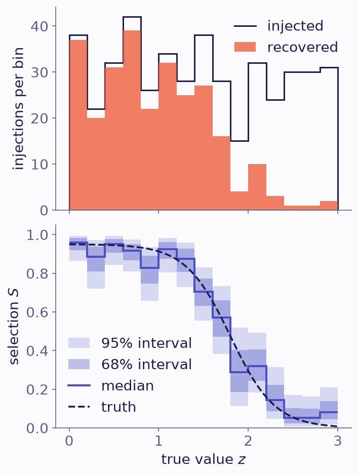
Injections give the selection with its uncertainty. Top: 450 injections, uniform in the true value, and the ones the pipeline recovered. Bottom: the posterior of \(S_k\) in each bin from those counts (Selection.from_injections), against the true completeness (dashed). Bins with few injections get wide bands.

binference then infers the selection together with the population. The catalogue’s objects count as detections in their bins, and the objects it missed as non-detections. The catalogue informs only the ratios between the \(S_k\): its likelihood does not change when all of them are scaled together. Their level, and with it the total, comes from the injections. The draws of \(S\) are in result.info["selection_draws"], and the total and the per-object methods use them draw by draw.

rng = np.random.default_rng(3)
z_inj = rng.uniform(0.0, 3.0, 600)
recovered = rng.random(600) < S[bins.index(z_inj)]     # the mock's S
measured = binference.Selection.from_injections(z_inj, recovered, bins, "on_truth")
joint = binference.infer(lk, selection=measured, method="nuts", n_samples=300, n_warmup=300, rng=1)
print(joint.mean.round(3), joint.info["selection_draws"].mean(axis=(0, 1)).round(2))

Gibbs, NUTS, Laplace and MAP(space="unconstrained") infer it; VB and the bootstrap do not (theory). For those, or to ignore the uncertainty, measured.at_mean() gives a fixed selection at its mean values. For a selection on the measurement, pass Selection.from_injections(...).at_mean(), a fixed selection; binference infers only a selection on the truth.

Few injections per bin

With few injections per bin, smooth=\(\tau_S\) lets neighbouring bins share information. It puts a second-order random walk on \(\mathrm{logit}\,S\), with step scale \(\tau_S\), and works on 1-D bins with every engine but Gibbs. Its values are the mode of \(\mathrm{logit}\,S\) given the injections. \(\tau_S\) is the typical change, from one bin to the next, of the slope of \(\mathrm{logit}\,S\) per bin.

Smoothing helps smooth completeness curves with few injections per bin, not sharp edges. A sharp edge needs independent bins or a larger \(\tau_S\).

smooth = binference.Selection.from_injections(z_inj, recovered, bins, "on_truth", smooth=0.3)
fit = binference.infer(lk, selection=smooth, method="laplace", n_samples=300, rng=1)
print(fit.mean.round(3), fit.info["selection_draws"].mean(axis=(0, 1)).round(2))

Totals and rates

Every fit of fractions also gives the total and the rates. Suppose \(W\) objects were detected, and \(S\) is absolute: detection probabilities, or exposures with scale="exposure". The number of detections is then Poisson with mean \(\Lambda\,S\cdot\rho\), where \(\Lambda\) is the total expected number of objects.

• The total. result.total holds one draw of \(\Lambda\) per draw of \(\rho\), under a scale-free prior on \(\Lambda\) (theory).

• The rates. result.rates holds \(\lambda_k=\Lambda\rho_k\): the expected number of objects per bin, per unit exposure.

• A relative selection identifies no total, and both are None.

• Non-integer weights give a pseudo-posterior for the total too (Advanced input options).

fit = binference.infer(
    lk, method="nuts", n_samples=300, n_warmup=300, rng=1,
    selection=binference.Selection(S, "on_truth", scale="exposure"),
)
print("total:", fit.total.mean().round(0), "+/-", fit.total.std().round(0),
      " actually drawn:", mock.truth.n_drawn)

The total inherits the prior on the fractions, which biases the total low when it is poorly determined, for example when some bins hold few detections (theory). Check a total’s calibration on simulations (Check a result) before you quote it from such data.

The objects the catalogue missed

result.realized_counts(full=True) draws the histogram of the full sample: the detected objects in their bins, plus the missed ones. For each draw, the number missed is negative binomial, and they fall in bins in proportion to \(\rho_k(1-S_k)\).

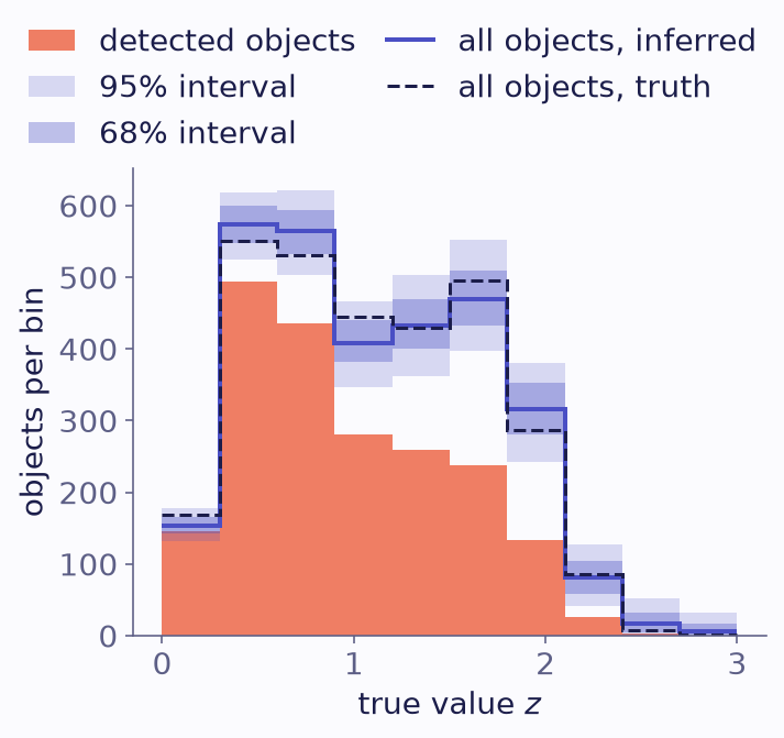
From detected counts to the full sample. 3000 objects were drawn and each was detected with a probability that falls from 0.95 to 0.15 across the bins. The fit sees the detected ones (filled) and the selection. The median with 68% and 95% bands of realized_counts(full=True) add the missed objects; the dashed line is the true histogram of all 3000.

In this example the fit saw 2013 detected objects, and its mean total is 3027 of the 3000 drawn.

Priors on the rates

To put a prior on the rates themselves, use GammaRates (rates instead of fractions). The selection then acts as an exposure in the same way.

est = binference.infer(
    lk, binference.priors.GammaRates(1.0, 1e-4), method="map",
    selection=binference.Selection(S, "on_truth", scale="exposure"),
)
print("expected total:", est.rates.sum().round(0), " actually drawn:", mock.truth.n_drawn)

Next

Two mistakes are common: correcting for the selection twice, and not at all (pitfall).

The selection tutorial and the populations-with-selection tutorial work through both modes and injections.