Tutorials / Selection effects and rates

Selection effects and rates

Catalogues are rarely complete. The selection \(S_k\) is the probability that an object in bin \(k\) enters the catalogue. This tutorial treats the two common cases, in the terms of the selection guide:

1. Occurrence rates, with a completeness that depends on the true value. The selection mode is "on_truth", with Poisson rates and an exposure.

2. A cut on the measured value, as in a flux-limited survey. The selection mode is "on_measurement".

import matplotlib.pyplot as plt
import numpy as np
from scipy import stats

import binference

rng = np.random.default_rng(2026)

1. Occurrence rates of planets

A simulated transit survey watches 5000 stars. Planet radii \(r_p\) are binned in \(\log_{10}(r_p/R_\oplus)\), with ten bins from 0.5 to 16 Earth radii. The occurrence rate \(\lambda_k\) is the expected number of planets per star in bin \(k\). The survey detects a planet with probability \(S_k\), which falls steeply for small planets. Measured radii scatter by 0.08 dex.

bins = binference.Bins.linear(np.log10(0.5), np.log10(16), 10)
log_radius = bins.centers
n_stars = 5_000
rate_true = 0.25 * np.exp(-0.5 * ((log_radius - 0.3) / 0.35) ** 2) + 0.02   # per star per bin
completeness = 1.0 / (1.0 + np.exp(-(log_radius - 0.1) / 0.12))          # detection probability

n_planets = rng.poisson(n_stars * rate_true)                          # all planets, per bin
edges = bins.edges[0]
true_log_r = np.concatenate([rng.uniform(edges[k], edges[k + 1], n)
                             for k, n in enumerate(n_planets)])
detected = rng.random(true_log_r.size) < completeness[bins.index(true_log_r)]
sigma = 0.08
obs_log_r = true_log_r[detected] + sigma * rng.standard_normal(detected.sum())
print(f"{n_planets.sum()} planets, {detected.sum()} detected")

7982 planets, 5726 detected

Detection depends on the true radius, not on the measurement, so the selection acts on the truth. To infer rates per star, the exposure is the number of stars \(N_\star\) times the completeness. The expected number of detections in bin \(k\) is then \(N_\star S_k\lambda_k\). The products \(N_\star S_k\) exceed one, so pass them as an exposure.

lk = binference.Likelihoods.from_gaussian(obs_log_r, sigma, bins)
fit = binference.infer(
    lk, binference.priors.GammaRates(shape=1.0, rate=1e-3),
    selection=binference.Selection(n_stars * completeness, "on_truth", scale="exposure"),
    rng=1,
)
idx = bins.index(obs_log_r)                                               # -1 outside the bins
naive = np.bincount(idx[idx >= 0], minlength=bins.K) / n_stars        # detected / stars

from binference.plotting import SAMPLE_COLOR
radius = 10 ** log_radius
mean = fit.rates.mean(axis=0)
lo, hi = fit.interval(0.68, which="rates")
fig, ax = plt.subplots()
fig.set_figheight(3.8)
ax.errorbar(radius, mean, yerr=[mean - lo, hi - mean], fmt="o", color="C0", ms=7,
            capsize=3, label="binference")
ax.plot(radius, rate_true, "k--", lw=1.5, label="truth")
ax.plot(radius, naive, "s", color=SAMPLE_COLOR, ms=7, label="detected / stars")
ax.set(xscale="log", yscale="log", xlabel=r"planet radius [$R_\oplus$]",
       ylabel="planets per star")
ax.legend(ncol=2, loc="lower left", bbox_to_anchor=(0, 1));

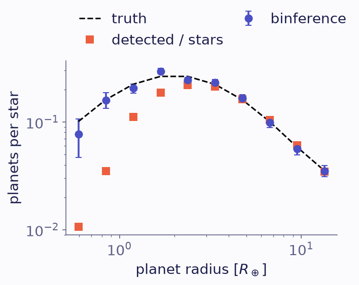
Occurrence rates per star in each radius bin. Circles with 68% intervals are inferred by binference; squares are detected planets per star; the truth is dashed.

Naive counts miss most small planets. binference’s rates agree with the truth, and their error bars are widest in the smallest bin, where few planets were detected:

sd = fit.rates.std(axis=0)
print("rate / its sd, per bin:", (mean / sd).round(1))

rate / its sd, per bin: [ 2.5  6.1 10.  16.6 15.4 15.7 13.   9.9  7.7  8.6]

Integrated quantities come from the draws:

small = log_radius < np.log10(2.0)
per_star = fit.rates[:, small].sum(axis=1)
print(f"planets smaller than 2 Earth radii per star: {per_star.mean():.3f} ± {per_star.std():.3f}"
      f"   (truth {rate_true[small].sum():.3f})")

planets smaller than 2 Earth radii per star: 0.736 ± 0.030   (truth 0.749)

2. A cut on the measured value

A flux-limited redshift survey keeps an object only if its measured redshift is below \(z_{\rm lim}=1.6\). Objects whose true redshift is just above the limit can scatter in, and objects just below it can scatter out.

zbins = binference.Bins.linear(0.0, 2.5, 25)
rho_true = binference.simulate.population(zbins, lambda z: z**2 * np.exp(-z / 0.4))
labels = rng.choice(zbins.K, size=2_500, p=rho_true)
ze = zbins.edges[0]
z_true = rng.uniform(ze[labels], ze[labels + 1])
sig_z = 0.12
z_obs = z_true + sig_z * rng.standard_normal(z_true.size)
keep = z_obs < 1.6
lk_z = binference.Likelihoods.from_gaussian(z_obs[keep], sig_z, zbins)
print(f"kept {keep.sum()} of {keep.size}")

kept 2023 of 2500

Here the selection acts on the measurement. \(S_k\) is the probability that an object in bin \(k\) passes the cut, averaged over the bin. These values are already bin averages, so they go in as a Selection object; infer checks a raw array for steep changes between bins.

fine = np.linspace(0, 2.5, 2501)
pass_prob = stats.norm.cdf((1.6 - fine) / sig_z)
S = np.array([pass_prob[(fine >= a) & (fine < b)].mean() for a, b in zip(ze[:-1], ze[1:])])

gp = binference.priors.LogisticGP()
kw = dict(rng=1, n_samples=400, n_warmup=300)
fits = {
    "selection on the measurement": binference.infer(
        lk_z, gp, selection=binference.Selection(S, "on_measurement"), **kw
    ),
    "no selection": binference.infer(lk_z, gp, **kw),
}

Both fits use a Gaussian-process prior. Beyond the cut the data say almost nothing. A smoothness prior extends the shape below the cut into those bins; under a Dirichlet prior they would be nearly unconstrained.

fig, axes = plt.subplots(2, 1, sharex=True, sharey=True)
fig.set_figheight(5.1)
for ax, (name, res) in zip(axes, fits.items()):
    res.plot(ax=ax, truth=rho_true, label="median")
    ax.set_title(name, loc="left")
    ax.axvline(1.6, color="0.45", lw=1, ls=":")
axes[0].get_legend().remove()
axes[1].legend(loc="upper right")
axes[0].set_xlabel("")
axes[1].set_xlabel("z");

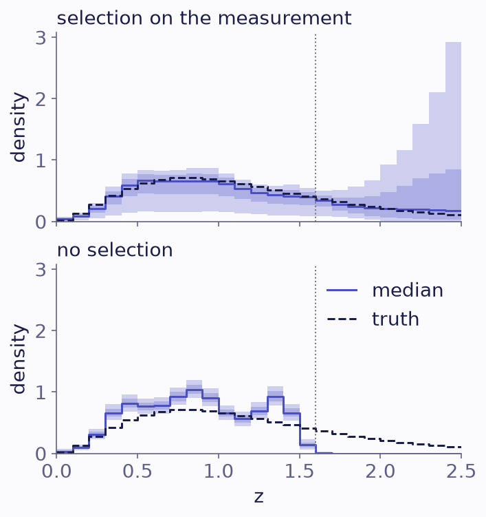
The redshift population (median, 68% and 95% bands) with the selection on the measurement (top) and without it (bottom). The dotted line marks the cut at 1.6; the truth is dashed.

Ignoring the cut truncates the population sharply at the limit. With the selection, the fit recovers the population in the three bins just beyond \(z_{\rm lim}\), from the objects that scattered across the cut:

beyond = (zbins.centers > 1.6) & (zbins.centers < 1.9)
for name, res in fits.items():
    print(f"{name:28s} fraction in 1.6-1.9: {res.functional(lambda r: r[beyond].sum()).mean():.3f}")
print(f"{'truth':28s} fraction in 1.6-1.9: {rho_true[beyond].sum():.3f}")

selection on the measurement fraction in 1.6-1.9: 0.087
no selection                 fraction in 1.6-1.9: 0.001
truth                        fraction in 1.6-1.9: 0.096

The smoothness prior carries the population further, and the widening bands show where the data run out.

Note

Passing "on_truth" here would be wrong. It would multiply each object’s likelihood by \(S_k\), as if objects were selected on their true redshift, and so count the selection twice. Always ask what the selection acts on.