Tutorials / Selection measured by injections

Selection measured by injections

Gravitational-wave detectors see heavy binary black holes to much larger distances than light ones. A catalogue of detections therefore over-represents heavy systems. The correction needs the detection probability \(S(m)\) at each mass \(m\), which is not known in closed form. It is measured with injections: simulated signals of known mass are added to the detector data, and the pipeline records which it recovers. Exoplanet surveys measure their completeness the same way.

Selection effects and rates uses a selection that is known exactly. Here a finite set of injections measures it, so it is uncertain. binference infers it together with the population (from_injections()). The tutorial compares three fits: one that ignores the selection, one that plugs in the injection estimate, and one that infers both together.

import matplotlib.pyplot as plt
import numpy as np
from scipy import stats

import binference

rng = np.random.default_rng(150914)

A simulated catalogue

The mergers follow the population of primary masses \(m\) in Posterior samples: black-hole masses: a power law with a peak at 34 solar masses. A merger is detected with probability \(S(m) = 0.8/[1 + (m/20)^{-3}]\). Detection is a random event, independent of the measurement error, so the selection acts on the true mass ("on_truth"). Each merger has a measured \(\ln m\) with a Gaussian error between 0.05 and 0.2. Gaussian likelihoods keep this tutorial about the selection.

The bins are 16 equal intervals in \(\ln m\). mock_1d draws the 6000 mergers and their measurements; the detected ones form the catalogue:

m_lo, m_hi, slope = 5.0, 85.0, -2.3

def population(x):                       # density of ln m, as in the posterior-samples tutorial
    m, a = np.exp(x), slope + 1
    power_law = a * m**slope / (m_hi**a - m_lo**a)
    return (0.9 * power_law + 0.1 * stats.norm.pdf(m, 34.0, 4.0)) * m

def S(m):                                # detection probability
    return 0.8 / (1 + (np.asarray(m) / 20.0) ** -3)

bins = binference.Bins.linear(np.log(m_lo), np.log(m_hi), 16)
n_mergers = 6000
mock = binference.simulate.mock_1d(n_mergers, bins, density=population, noise=(0.05, 0.2),
                                   rng=rng)
rho_true = mock.truth.rho
detected = rng.random(n_mergers) < S(np.exp(mock.truth.values))
lk = binference.Likelihoods.from_gaussian(
    mock.measurements["mean"][detected], mock.measurements["sigma"][detected], bins,
    warn_outside=False,                  # measurements near the edges spill past them
)
print(f"{n_mergers} mergers, {detected.sum()} detected")

6000 mergers, 1250 detected

The injection campaign

The campaign injects 3000 signals with masses drawn uniformly in \(\ln m\). Each is recovered with probability \(S(m)\). In the lightest bins only a few injections are recovered, so the detection probability there is known only roughly. Selection.from_injections tallies the injected and recovered signals per bin, \(n^{\rm inj}_k\) and \(n^{\rm rec}_k\). It gives each bin’s detection probability \(S_k\) a Beta posterior (selection guide). sel.injections holds the tallies.

n_inj = 3000
m_inj = np.exp(rng.uniform(np.log(m_lo), np.log(m_hi), n_inj))
found = rng.random(n_inj) < S(m_inj)
sel = binference.Selection.from_injections(np.log(m_inj), found, bins, "on_truth")
injected, recovered, (a_prior, b_prior), _ = sel.injections
print("recovered / injected, lightest five bins:",
      [f"{r:.0f}/{n:.0f}" for r, n in zip(recovered[:5], injected[:5])])

recovered / injected, lightest five bins: ['3/173', '6/168', '5/184', '14/188', '17/180']

Four fits

1. No selection. The catalogue is treated as a fair sample.

2. Plug-in. The injection estimate sel.at_mean() is used as if it were exact.

3. Joint. The detection probabilities are inferred together with the population, from the injections and the catalogue.

4. Exact. For reference, the true \(S(m)\) averaged over each bin (from_function()). A real analysis does not have it.

All four use NUTS, so that they are comparable. In the joint model, the population fractions and the detection probability are correlated in the lightest bins, where there are few detections: a higher detection probability allows a lower fraction.

exact = binference.Selection.from_function(lambda x: S(np.exp(x)), bins, "on_truth")
kw = dict(method="nuts", n_warmup=500, rng=1)
fits = {
    "no selection": binference.infer(lk, **kw),
    "plug-in injections": binference.infer(lk, selection=sel.at_mean(), **kw),
    "joint": binference.infer(lk, selection=sel, **kw),
    "exact selection": binference.infer(lk, selection=exact, **kw),
}
d = fits["joint"].diagnostics
print(f"joint fit: max R-hat {d['rhat'].max():.3f}, min bulk ESS {d['ess_bulk'].min():.0f}, "
      f"selection max R-hat {d['rhat_selection'].max():.3f}, divergent {d['n_divergent']}")

joint fit: max R-hat 1.004, min bulk ESS 1306, selection max R-hat 1.004, divergent 0

fig, axes = plt.subplots(3, 1, sharex=True, sharey=True)
fig.set_figheight(7.2)
for ax, name in zip(axes, ["no selection", "plug-in injections", "joint"]):
    fits[name].plot(ax=ax, which="fractions", truth=rho_true, label="median")
    ax.set_title(name, loc="left")
    ax.set_xlabel("")
    ax.get_legend().remove()
axes[1].legend(loc="upper right")
axes[-1].set_xlabel(r"$\ln(m / M_\odot)$");

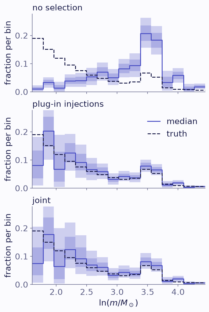
Population fractions of the primary mass, with 68% and 95% bands. The fits ignore the selection (top), plug in the injection estimate (middle), or infer it jointly (bottom). The truth is dashed.

Ignoring the selection gives the population of detections, which is heavily weighted toward high masses. Both corrected fits recover the shape. They differ in the lightest bins, where few injections were recovered: the joint fit’s bands are wider there.

Derived quantities

Two derived quantities depend most on the lightest bins. One is the fraction of mergers in the four lightest bins, below 10.2 solar masses. The other is the total number of mergers \(\Lambda\), including those never detected (result.total):

light = np.arange(bins.K) < 4                  # upper edge at 10.15 Msun
frac = {name: res.functional(lambda rho: rho[light].sum()) for name, res in fits.items()}
print(f"{'':20s} fraction below 10.2 Msun total mergers")
for name, res in fits.items():
    f = frac[name]
    print(f"{name:20s} {f.mean():.3f} ± {f.std():.3f}            "
          f"{res.total.mean():6.0f} ± {res.total.std():4.0f}")
print(f"{'truth':20s} {rho_true[light].sum():.3f}                    {n_mergers:6d}")

                     fraction below 10.2 Msun total mergers
no selection         0.097 ± 0.010              1250 ±   35
plug-in injections   0.487 ± 0.034              5166 ±  318
joint                0.466 ± 0.055              5025 ±  550
exact selection      0.538 ± 0.032              5788 ±  355
truth                0.556                      6000

Without a selection, the total is just the number of detections. The joint fit’s error bars are larger than the plug-in fit’s. They include the uncertainty of the detection probability from a finite number of injections, which the plug-in fit treats as exact. Both totals fall below the truth: the plug-in total by 2.6 of its standard deviations, the joint total by 1.8 of its own.

A total this poorly determined also depends on the prior, which by default biases it low (selection guide). Before you quote a total from such data, check its calibration on simulations (Validating an analysis).

The joint fit also returns posterior draws of the detection probability, info["selection_draws"]. The catalogue informs only the ratios between bins, so the level comes from the injections:

S_draws = fits["joint"].info["selection_draws"].reshape(-1, bins.K)
S_lo, S_hi = np.quantile(S_draws, [0.05, 0.95], axis=0)
beta = stats.beta(a_prior + recovered, b_prior + injected - recovered)
fine = np.linspace(np.log(m_lo), np.log(m_hi), 400)

fig, ax = plt.subplots()
fig.set_figheight(3.8)
ax.plot(fine, S(np.exp(fine)), "k--", lw=1.2, label="truth")
for dx, mid, lo, hi, color, marker, label in [
    (-0.02, beta.mean(), beta.ppf(0.05), beta.ppf(0.95), "C1", "s", "injections alone"),
    (0.02, S_draws.mean(axis=0), S_lo, S_hi, "C0", "o", "joint fit"),
]:
    ax.errorbar(bins.centers + dx, mid, yerr=[mid - lo, hi - mid], fmt=marker, color=color,
                ms=6, capsize=2, label=label)
ax.set(xlabel=r"$\ln(m / M_\odot)$", ylabel="detection probability", yscale="log")
ax.legend(ncol=2, loc="lower left", bbox_to_anchor=(0, 1));

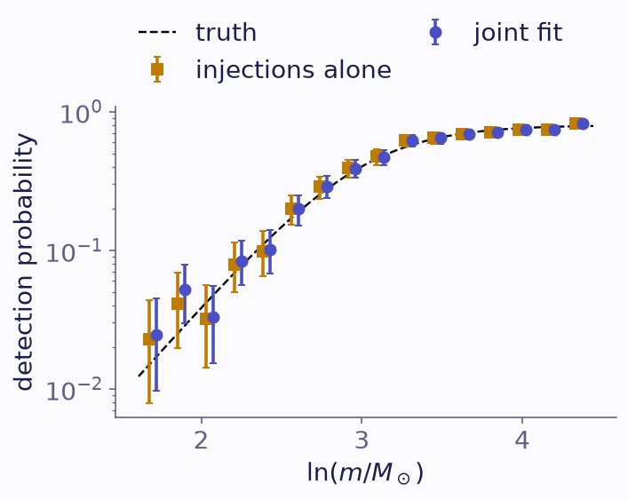
The detection probability per bin, with 90% intervals. Squares use the injections alone, circles the joint fit; the dashed line is the true S(m).

What to take away

• Selection.from_injections passed to infer infers the selection together with the population. sel.at_mean() is a plug-in that ignores the selection’s uncertainty, which is large where few injections are recovered.

• Here detection depends only on the true mass, so "on_truth" is exact. In real detectors, detection and measurement share the same noise, and the selection acts on the measurement (Selection effects and rates shows the difference). The gravitational-wave background page says what that means for a selection measured by injections.