Concepts / Bins and likelihoods

Bins and likelihoods

What does binference need to know about each object, and why does it work with bins?

Objects and bins

You have \(N\) objects: galaxies, events, patients or documents. Each object \(i\) has data \(d_i\), such as a measured flux or a classifier’s score. Each object also has a true value \(z\) that you never see exactly, such as a redshift or a class.

binference divides the range of \(z\) into \(K\) bins \(B_1,\dots,B_K\). A bin can be an interval, a cell of a grid, or a category. Its bin volume \(v_k\) is its width in one dimension, its area on a grid, and one for a category.

One object’s likelihood

The likelihood function \(\ell_i(z)=p(d_i\mid z)\) says how probable object \(i\)’s data are if its true value is \(z\). It is not a distribution over \(z\), and its overall scale does not matter: only its shape across \(z\) carries information.

The model uses one number per object and bin, the bin-averaged likelihood. On linear bins it is

\[ L_{ik}=\frac{1}{v_k}\int_{B_k}\ell_i(z)\,dz , \]

the average of \(\ell_i\) over bin \(k\) (the measures section below covers other bins). The \(N\times K\) table of these numbers is the likelihood matrix. Explainer V-1 below shows one object’s likelihood and its bin averages for any error and bin width.

V-1 · Bin averages of one likelihood

error σ

0.20

bin width

0.25

3 bins hold more than 5% of the likelihood

One object measured at \(d_i=1.37\) with a Gaussian error \(\sigma\). The dashed curve is the likelihood \(\ell_i(z)\); the steps are its bin averages \(L_{ik}\), the same numbers Likelihoods.from_gaussian computes. Move the sliders: a narrow likelihood puts almost all its weight in one or two bins, a broad one spreads it over many.

When the likelihood is much narrower than the bins, each object places nearly all its likelihood in one bin. When it is broader, it spreads over several bins, and the data cannot say which of them the object lies in. The population page shows what that does to the fit.

Why bins

The population is a histogram: a fraction \(\rho_k\) of it lies in bin \(k\), spread evenly within the bin. Under that assumption, the probability of object \(i\)’s data is a dot product,

\[ p(d_i\mid\rho)=\sum_k\rho_k L_{ik}=L_i\cdot\rho . \]

Every input type reduces to such a table. Gaussian measurements, posteriors, posterior samples, counts in measured bins and classifier outputs all become rows \(L_i\). One model then handles all of them, and the cost of a fit grows with \(N\times K\) whatever the input was.

Masses versus densities

\(L_{ik}\) is an average over the bin, a value per unit volume. Inputs often come as values integrated over each bin instead, such as differences of a cumulative distribution or histograms of samples. The first kind is a density, the second a mass, and a mass equals the density times the bin volume.

With equal bins the two differ by one constant, which cancels. With unequal bins they have different shapes. If you pass masses as densities, the peak moves toward the widest bins (the mass figure). Say which you pass, as the inputs guide shows.

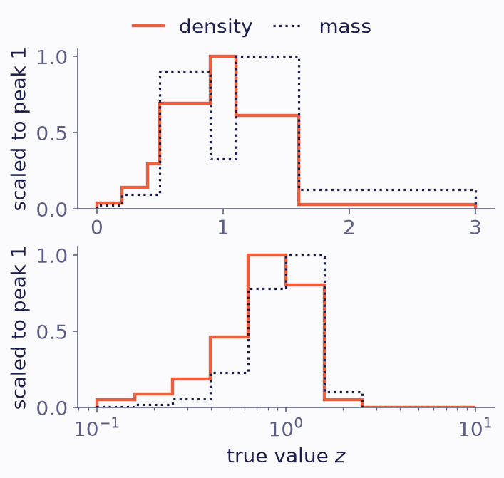
One object’s likelihood, Gaussian with mean 1 and standard deviation 0.35. It is shown as bin averages (density, solid) and bin integrals (mass, dotted), each scaled to a peak of one. Top: unequal bins on a linear axis. Bottom: ten log-spaced bins from 0.1 to 10 on a logarithmic axis. The density follows the likelihood; the mass peaks in a wide bin.

Measures: flat in which coordinate?

The model takes the population as flat within each bin. Flat needs a coordinate, and binference calls it the bin axis’s measure, \(u=T(z)\). Linear bins use \(u=z\). Logarithmic bins use \(u=\log z\), so the population is flat in \(\log z\) within each bin. A logarithmic bin’s centre is then the geometric mean of its edges.

With a measure other than \(u=z\), binference averages \(\ell_i\) over each bin uniformly in \(u\), and the population is flat in \(u\), not in \(z\). The measure also decides what a smoothness prior calls flat (see priors on the simplex). Choose the coordinate in which the population changes least across a bin.

When the population is not flat within the bins, the resulting binning bias does not shrink as you add objects; the inputs guide shows how a within-bin basis reduces it.

In plain words

binference asks one question of each object: how well does each bin explain its data? The answers, one per bin, are all it needs.

Where next

• Do it: the inputs guide.

• See it: the tutorial Posteriors on a grid.

• Derivation: objects, bins and likelihoods in How it works.