Tutorials / Posteriors on a grid

Posteriors on a grid

Many surveys publish each object’s posterior on a grid of bins rather than its likelihood. A photometric-redshift code, for example, reports \(P_{ik}\): the mass of object \(i\)’s posterior in bin \(k\). Each posterior was computed under some prior, the interim prior \(\pi\). This tutorial shows how to tell binference what the table holds: the prior to divide out, and whether the numbers are masses or densities.

import matplotlib.pyplot as plt
import numpy as np

import binference

bins = binference.Bins.linear(0.0, 3.0, 20)

Posteriors under an interim prior

mock_1d(interim="gaussian") also returns what a photometric-redshift code would report. Each object’s posterior is computed under a broad Gaussian interim prior centred at \(z=1.8\), far from the true population. mock.interim holds the prior’s mass in each bin, \(\Pi_k\).

mock = binference.simulate.mock_1d(2000, bins, noise=(0.2, 0.4), interim="gaussian", rng=3)
P, interim = mock.posteriors, mock.interim
print(P.shape, "rows sum to", P.sum(axis=1)[:3].round(6))

(2000, 20) rows sum to [1. 1. 1.]

The right way passes the interim prior, so that binference divides it out. The tempting way feeds the posteriors in as if they were likelihoods. Both fits use a smoothness prior, whose narrow bands make the difference easy to see:

prior = binference.priors.LogisticGP()
kw = dict(rng=1, n_samples=400, n_warmup=400)   # shorter runs than the default, for speed
right = binference.infer(binference.Likelihoods.from_table(P, bins, interim=interim), prior, **kw)
wrong = binference.infer(binference.Likelihoods(P, bins), prior, **kw)

ip = interim / bins.volumes
fig, axes = plt.subplots(2, 1, sharex=True, sharey=True)
fig.set_figheight(5.6)
right.plot(ax=axes[0], truth=mock.truth.rho, label="median")
wrong.plot(ax=axes[1], truth=mock.truth.rho, color="C1", label="median")
for ax, title in zip(axes, ["interim prior divided out", "posteriors used as likelihoods"]):
    ax.step(bins.edges[0], np.append(ip, ip[-1]), where="post", color="0.45", lw=1,
            label="interim prior")
    ax.set_title(title, loc="left")
    ax.get_legend().remove()
fig.legend(*axes[0].get_legend_handles_labels(), loc="outside lower center", ncol=2)
axes[0].set_xlabel("")
axes[1].set_xlabel("z");

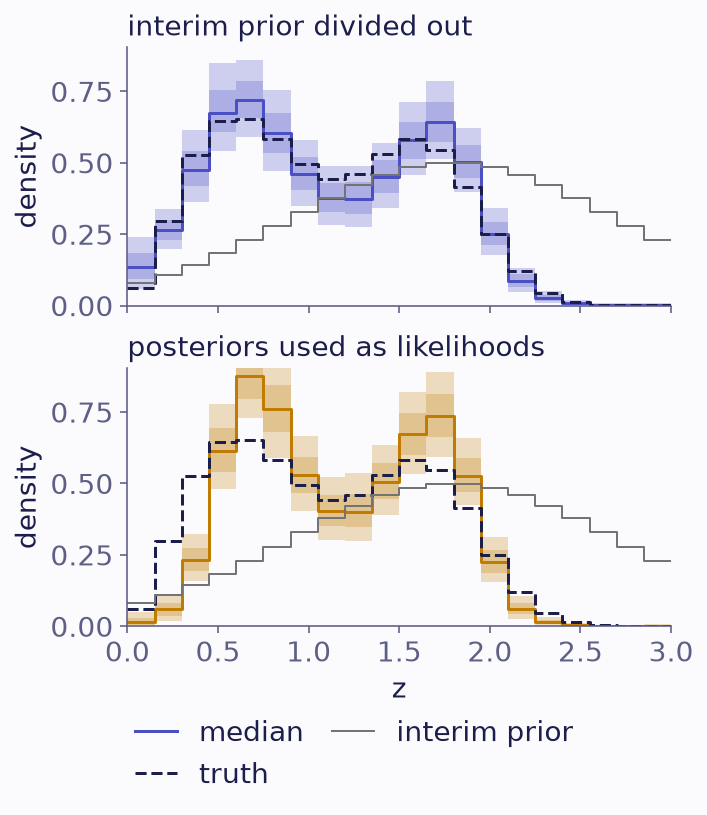
Fits that divide out the interim prior (top) and that use the posteriors as likelihoods (bottom), with 68% and 95% bands. The thin grey line is the interim prior; the truth is dashed.

Using the posteriors directly counts the interim prior twice. The population shifts toward where that prior is large. The error bars give no warning: the wrong answer is just as confident.

for name, fit in [("right", right), ("wrong", wrong)]:
    zbar = fit.functional(lambda rho: rho @ bins.centers)
    print(f"mean redshift, {name} fit: {zbar.mean():.3f} ± {zbar.std():.3f}")
print(f"mean redshift, truth:     {mock.truth.rho @ bins.centers:.3f}")
z_wrong = (wrong.mean - mock.truth.rho) / wrong.std
print("largest bias of the wrong fit:", np.abs(z_wrong).max().round(1), "posterior sd")
z_right = (right.mean - mock.truth.rho) / right.std
print("largest deviation of the right fit:", np.abs(z_right).max().round(1), "posterior sd")

mean redshift, right fit: 1.105 ± 0.014
mean redshift, wrong fit: 1.175 ± 0.014
mean redshift, truth:     1.110
largest bias of the wrong fit: 10.2 posterior sd
largest deviation of the right fit: 1.7 posterior sd

If the code’s prior was flat, pass interim="flat". If you do not know the prior, ask the team that made the table, because binference cannot recover it from the posteriors.

Masses or densities

The model needs bin-averaged likelihoods, so a table of masses must be divided by the bin widths (masses versus densities). With equal bins the difference cannot matter. With unequal bins it does.

Here five unequal bins hold 5000 objects. Their posteriors under a flat prior are given as masses, the differences of the Gaussian distribution function across each bin:

from scipy import stats

ubins = binference.Bins([0.0, 0.25, 0.5, 1.0, 2.0, 3.0])
rho_true = np.array([0.15, 0.25, 0.3, 0.2, 0.1])
umock = binference.simulate.mock_1d(5000, ubins, density=rho_true, noise=0.15, rng=4)
mu, sig = umock.measurements["mean"], umock.measurements["sigma"]

edges = ubins.edges[0]
cdf = stats.norm.cdf((edges[None, :] - mu[:, None]) / sig[:, None])
masses = np.diff(cdf, axis=1)                  # posterior mass in each bin

as_masses = binference.infer(binference.Likelihoods.from_table(masses, ubins, interim="flat"),
                             method="map").rho
as_densities = binference.infer(binference.Likelihoods(masses, ubins), method="map").rho
print("truth          ", rho_true)
print("masses (right) ", as_masses.round(3))
print("densities      ", as_densities.round(3))
print("bin widths     ", ubins.volumes)

truth           [0.15 0.25 0.3  0.2  0.1 ]
masses (right)  [0.16  0.244 0.295 0.2   0.101]
densities       [0.213 0.083 0.388 0.216 0.1  ]
bin widths      [0.25 0.25 0.5  1.   1.  ]

Read as densities, the masses distort the population. Mass moves from the narrow second bin into its neighbours, by far more than the statistical error of 5000 objects. from_table with an interim prior reads the table as masses by default; the inputs guide gives the other representation.

What to take away

• Pass the interim prior with the posteriors: Likelihoods.from_table(P, bins, interim=interim).

• Say whether the table holds masses or densities whenever the bins are unequal.

• The inputs guide lists the forms an interim prior can take. Posterior samples: black-hole masses starts from samples instead of a table.