Concepts / Engines

Engines

binference offers several engines. What does each one compute, and when is its answer exact?

One posterior, several ways to reach it

The model fixes one posterior for the population, \(p(\rho\mid D)\). An engine is an algorithm that describes it. This table is the summary of what each engine computes and when its answer is exact.

engine	computes	exact when
NUTS	draws from the posterior	always, once its chains have converged
Gibbs	draws from the posterior, with every object’s bin	for a conjugate prior and integer weights, once converged
MAP	the most probable population, with a certificate	never; it is a point, not a posterior
Laplace	draws from a heavy-tailed version of a Gaussian at the mode, reweighted toward the posterior	when its importance check passes
mean-field VB	draws from an approximation that treats the population and the objects’ bins as independent	never; its intervals are too narrow
bootstrap	MAP estimates refitted to resampled objects	never; it is not a posterior
auto	Gibbs, Laplace or NUTS, chosen for the data	when the engine it chose is

binference marks results whose draws are not from the exact posterior as approximate.

The engines one by one

NUTS. NUTS follows the slope of the log posterior to take long steps through it. It works with every prior, and its draws stay nearly independent even when likelihoods are broad. R-hat, the effective sample size and its divergences check that its chains have converged.

Gibbs. Gibbs sampling alternates two exact steps. It draws every object’s bin given the population, then the population given those bins. When likelihoods are broad compared with the bins, each step changes the population only a little, so successive draws are strongly correlated. The missing information \(f\) measures this.

MAP. With the default flat Dirichlet prior, the MAP is the maximum-likelihood population. Three solvers share the work; the engines guide says which runs when. Its certificate, the KKT gap, says how close the answer is to the optimum. A point carries no uncertainty, so use it for quick looks and as a starting point.

Laplace. The Laplace engine fits a Gaussian at the posterior’s mode, in unconstrained coordinates, where every vector of real numbers is a valid population. It then draws from a heavy-tailed version of that Gaussian and reweights the draws so that they follow the exact posterior (importance sampling). The Pareto k-hat \(\hat k\) of the weights says whether that worked. If it did not, binference marks the result approximate.

Mean-field VB. Treating the population and each object’s bin as independent ignores the coupling that broad likelihoods create. That is why its intervals are too narrow. It is fast, and binference always marks the result approximate.

Bootstrap. The bootstrap refits the MAP to resampled or reweighted objects. It answers how much the estimate would change with new data, not how probable each population is.

Auto. The default engine tries Gibbs where Gibbs mixes well enough, running it longer to make up for correlated draws. It then tries Laplace where its check passes, and NUTS otherwise. Auto gives the thresholds. The rules, and the benchmark behind them, are in how auto chooses.

Seeing them on one problem

Figure shows a population on three bins. The fractions \((\rho_1,\rho_2,\rho_3)\) lie on a triangle, and unconstrained coordinates \((x_1,x_2)\) map that triangle to the whole plane. The samplers and the approximations describe the same posterior there, and MAP marks its highest point.

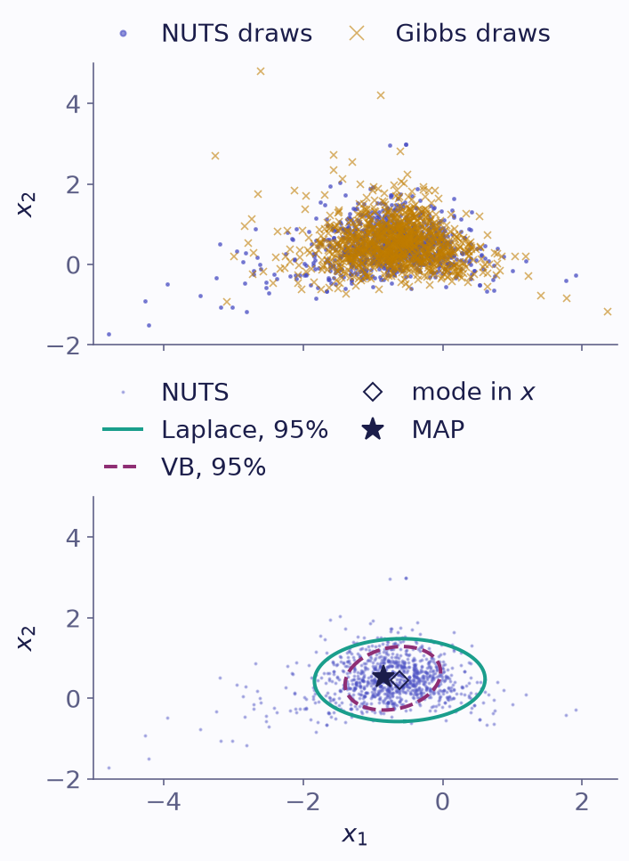
One posterior of a population on three bins, in unconstrained coordinates \(x\). It comes from 40 mock objects with measurement errors between 0.4 and 0.8. Top: 1,000 draws each from NUTS and Gibbs, two chains each. Bottom: the NUTS draws and the 95% ellipses of the Laplace Gaussian and of mean-field VB. The diamond is the mode in \(x\), where the Laplace Gaussian is centred. The star is the MAP on the simplex.

NUTS and Gibbs agree: both draw from the exact posterior. The missing information here is \(f=\) 0.78, so successive Gibbs draws are correlated, but the chains still mix. The Laplace Gaussian is symmetric, while the posterior has a longer tail to one side. Here its importance check passed, with \(\hat k=\) 0.01 against a limit of 0.70, so its reweighted draws follow the posterior. The mean-field VB ellipse is too small. Its standard deviations are 0.54 times those of NUTS (median over the fractions).

The MAP and the mode in \(x\) differ because they are the peaks of two densities of the same posterior, one in \(\rho\) and one in \(x\).

In plain words

NUTS and Gibbs draw from the posterior, and Laplace and VB approximate it; binference marks an approximation that is not exact. MAP finds the posterior’s highest point. The bootstrap answers a different question.

Where next

• Do it: the engines guide.

• See it: the tutorial Choosing an engine.

• Derivation: the engines in How it works.