Concepts / Population and objects

Population and objects

What does binference infer: the population, the objects you observed, or each object’s true value?

It infers the first two, and a posterior for the third. This page separates them.

The population and the realised sample

The population is the distribution the objects are drawn from. binference describes it by the population fractions \(\rho_k\), the share of the population in bin \(k\). The fractions are non-negative and sum to one, so they lie on the simplex \(\Delta^{K-1}\). On linear bins the population density within bin \(k\) is \(p(z\mid\rho)=\rho_k/v_k\); with another measure it is flat in that coordinate instead.

Your \(N\) objects are one draw from that population. Their histogram of true values is the realised sample \(n_k\). A second draw of \(N\) objects would give a different histogram, and each object’s data add measurement noise on top (the sample figure).

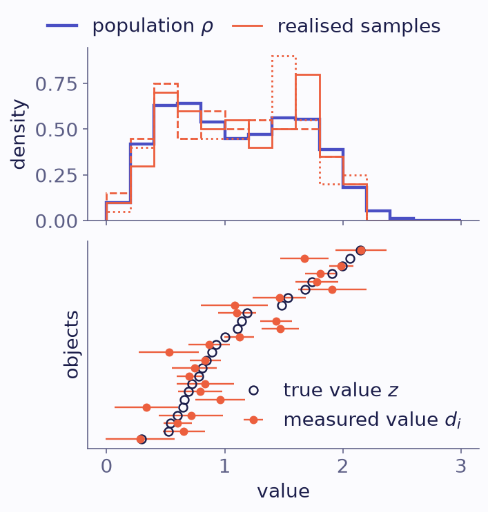
Top: a population on 15 bins (indigo). The coral lines are the histograms of three samples of 100 objects drawn from it. Bottom: 25 objects of one sample, sorted by true value. Each has a true value (open circle) and a measured value with its error bar (filled).

A property of the population, such as an occurrence rate or a luminosity function, needs \(\rho\). A property of these particular objects, such as the redshift distribution of one lens sample, needs \(n_k\). The uncertainty of \(n_k\) leaves out the noise of drawing \(N\) objects, so it is narrower. With perfect measurements \(n_k\) is known exactly, while \(\rho\) is still uncertain.

Stacking and the hierarchical fit

Each object’s posterior over bins, given a population \(\rho\), is its set of responsibilities:

\[ r_{ik}(\rho)=\frac{L_{ik}\rho_k}{L_i\cdot\rho}. \]

Averaging them over the objects gives a new estimate of the population. Starting from a flat population, the first average is the stack of the objects’ posteriors under a flat prior. EM repeats the average under each new estimate (explainer V-4). Each step removes more of the widening caused by measurement errors.

V-4 · Stacking, then EM

EM step

1

step 1 is the stack: mean log-likelihood per object −1.041

800 mock objects on 20 bins, measured with error 0.3. Indigo: the population after the chosen number of EM steps from a flat one; grey: step 1, the stack; dashed: the true population. Step forward and the two peaks sharpen; by step 200 the estimate swings between neighbouring bins.

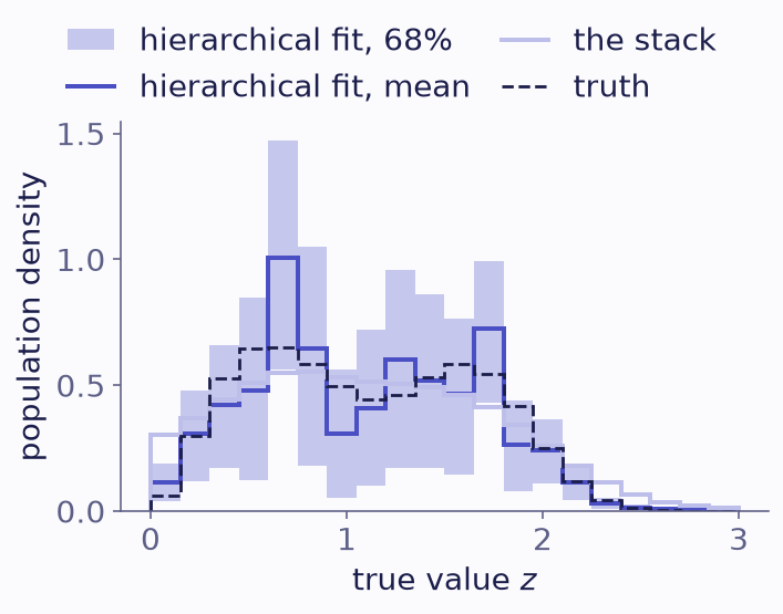
2,000 mock objects on 20 bins, with measurement errors between 0.15 and 0.35. Indigo: the hierarchical fit, the posterior mean and 68% band from Gibbs, four chains of 1,000 draws. Pale: the stack. Dashed: the true population.

Run to convergence, EM reaches the most probable population, the MAP. A hierarchical fit goes further: it gives the posterior of the population, with its uncertainty (the hierarchical-fit figure). The stack does neither. It is one step of the iteration, too smooth wherever the likelihoods are broader than the features of the population. The later EM steps in explainer V-4 turn jagged, for the reason the next section gives.

Correlations between bins

When likelihoods are broader than the bins, the data constrain the sum of neighbouring bins better than either bin. Mass can shift between them with little change in the likelihood, so their fractions are anti-correlated. In the fit of the hierarchical-fit figure, the median correlation between neighbouring bins is -0.57. Per-bin error bars therefore do not combine like independent errors; the pitfalls guide shows how to combine them.

Shrinkage: each object under the population

The population also informs each object. Let \(k_i\) be the bin of object \(i\), and \(D\) the data of all objects. Object \(i\)’s hierarchical posterior \(P(k_i=k\mid D)\) is its responsibilities averaged over the posterior of \(\rho\). It is narrower than the object’s own likelihood wherever the population is informative. This is shrinkage, and it is strongest when the population is narrow compared with the measurement error (explainer V-5).

V-5 · Shrinkage toward the population

population width

0.35

measured at 1.9; posterior mean 1.50

One object measured at 1.9 with error 0.4, on 30 bins, under a population centred at 1.2 (indigo). Its posterior \(r_{ik}(\rho)\) (solid coral) is its likelihood (dashed) times the population, normalised; each curve has unit area. Narrow the population and the posterior moves toward it; widen it and the posterior returns to the likelihood.

Shrinkage is not a bias to remove. Each object’s own likelihood leaves out where the other objects lie; the hierarchical posterior adds it.

In plain words

The population is where objects like yours come from, and your catalogue is one draw from it. binference estimates both, and where each object probably lies given the population.

Where next

• Do it: the results guide reads the population, individual objects and the realised sample from a fit.

• See it: the tutorial Gaussian measurements: a redshift distribution.

• Derivation: the augmented form in How it works.