
Concepts / Likelihoods and posteriors
Likelihoods and posteriors
Many codes report each object’s posterior instead of its likelihood. What is the difference, and why does it matter for the population?
A posterior contains a prior
A photometric-redshift code, a classifier or a per-object fitter usually returns a posterior for each object. It multiplies the object’s likelihood function by a prior and normalises:
The prior \(\pi\) is the interim prior. The code chose it before anyone knew the population. For a classifier, it is the class mix of the training set.
The same likelihood gives different posteriors under different interim priors (figure). A broad interim prior barely changes the likelihood. A narrow one moves the posterior toward its own peak.
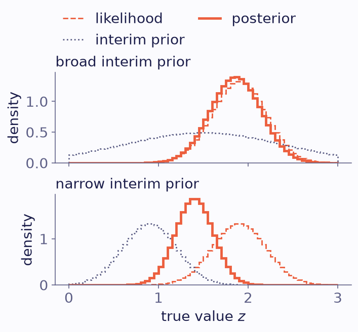
One object’s likelihood (dashed) times an interim prior (dotted) gives its posterior (solid), on 60 bins. The likelihood is Gaussian with mean 1.9 and standard deviation 0.3. Top: a broad interim prior, normal with mean 1.5 and standard deviation 0.9. Bottom: a narrow one, normal with mean 0.9 and standard deviation 0.3. Each curve has unit area.
Dividing the interim prior out
The population model needs likelihoods. If \(P_{ik}\) is the mass of object \(i\)’s posterior in bin \(k\), and \(\Pi_k\) the mass of the interim prior there, then
provided \(\pi\) is roughly constant within each bin. binference does this division for you. It has no default interim prior for posteriors or posterior samples, so you must name the one that was used.
Posteriors used as likelihoods
Treating posteriors as likelihoods counts the interim prior once per object. The data then constrain the product of \(\pi\) and the population rather than the population itself. The fit then favours populations that are large where \(\pi\) is large. It moves toward the interim prior, more so the narrower \(\pi\) is (explainer V-3). With uninformative data it equals the interim prior’s peak.
V-3 · Posteriors used as likelihoods
mean z: truth 1.38, prior divided out 1.37, posteriors as likelihoods 1.74
Population fits to 2,000 mock objects on 15 bins, measured with error 0.3, whose posteriors use a Gaussian interim prior (grey). Each fit is 50 EM steps from a flat population. Indigo: the interim prior divided out. Amber: the posteriors used as likelihoods. Dashed: the true population. Move or narrow the interim prior: the amber fit follows it, the indigo fit does not.
Stacking is one step from the interim prior
Stacking averages the objects’ posteriors and calls the average the population. The stack is one step of EM started from the interim prior, so it leans toward \(\pi\); explainer V-4 on the population page steps through the iterations that follow.
In plain words
A posterior is a likelihood with someone else’s guess about the population already mixed in. Take that guess out before you ask what the population is.
Where next
Do it: the inputs guide converts posteriors with their interim prior.
See it: the tutorial Posteriors on a grid repeats the comparison of explainer V-3 with a photometric-redshift mock.
Derivation: likelihoods versus posteriors in How it works.