Tutorial 1: Individual Star Models
EEPTracks, StarEvolTrack, and FastNNPredictor map stellar evolutionary and physical parameters (mini, eep, feh, afe, smf, av, rv, dist) to physical properties and multi-band photometry.
Topics Covered
EEPTracks for parameter prediction along evolutionary tracks
StarEvolTrack for on-the-fly SED generation
Exploring parameter space (mass, metallicity, age)
Binary star modeling
Extinction and distance effects
FastNNPredictor as a lightweight alternative to StarEvolTrack
Prerequisites
The setup cell below checks the data files this tutorial needs; Tutorial 00 shows how to download them.
# Optional: Download required data files (only needed if not already cached)
# This tutorial requires MIST evolutionary tracks and the C3K neural network.
# Uncomment the lines below to download them.

# from brutus.data import fetch_tracks, fetch_nns
# fetch_tracks()
# fetch_nns()
# Imports and setup
import numpy as np
import matplotlib.pyplot as plt
import warnings
warnings.filterwarnings('ignore')

from tutorial_utils import (
    setup_tutorial,
    print_saved_files,
    find_brutus_data_file,
    save_figure as _save_fig,
    print_section,
)

info = setup_tutorial(1, title="Tutorial 01: Individual Star Models")


def save_figure(fig, name):
    """Save figure to this tutorial's plot directory."""
    _save_fig(fig, 1, name)
Section 1: EEPTracks - Parameter Prediction
EEPTracks provides stellar parameter predictions along evolutionary tracks. It interpolates MIST stellar evolution models to predict physical parameters at any point along a star’s evolution.
Key Concepts
EEP (Equivalent Evolutionary Point): A normalized coordinate along stellar evolution tracks
Tracks vs Isochrones: Tracks follow individual stars, isochrones are snapshots of populations
Parameter prediction: Get stellar properties (Teff, log g, luminosity) at any EEP
from brutus.core import EEPTracks
from brutus.data import filters

# Initialize EEPTracks
mistfile = find_brutus_data_file("MIST_1.2_EEPtrk.h5")

tracks = EEPTracks(mistfile=mistfile, verbose=False)

# Explore the parameter space covered
masses = tracks.xgrid[0]  # Initial masses
metallicities = tracks.xgrid[2]  # [Fe/H] values

print(f"Loaded tracks covering {len(masses)} mass points")
print(f"  Mass range: {masses.min():.2f} - {masses.max():.2f} M☉")
print(f"  Metallicity range: {metallicities.min():.2f} - {metallicities.max():.2f}")
print(f"  Available predictions: {[str(p) for p in tracks.predictions]}")
Loaded tracks covering 188 mass points
  Mass range: 0.10 - 300.00 M☉
  Metallicity range: -4.00 - 0.50
  Available predictions: ['loga', 'logl', 'logt', 'logg', 'feh_surf', 'afe_surf', 'agewt']
# Predict parameters for a solar-mass star at different evolutionary stages
print("Predicting parameters for a 1 M☉ star at different evolutionary stages:")

# MIST primary EEPs (Dotter 2016) and points between them
eep_examples = [
    (202, "Zero-Age Main Sequence"),
    (353, "Intermediate-Age MS"),
    (454, "Terminal-Age Main Sequence"),
    (500, "Subgiant/Red Giant Branch"),
    (605, "Tip of the RGB"),
    (650, "Core Helium Burning")
]

for eep, phase in eep_examples:
    try:
        # get_predictions takes [mini, eep, feh, afe]
        params = tracks.get_predictions([1.0, eep, 0.0, 0.0])

        # Extract specific parameters (indices based on tracks.predictions)
        loga_idx = tracks.predictions.index("loga")
        logl_idx = tracks.predictions.index("logl")
        logt_idx = tracks.predictions.index("logt")
        logg_idx = tracks.predictions.index("logg")

        age_gyr = 10**params[loga_idx] / 1e9
        luminosity = 10**params[logl_idx]
        teff = 10**params[logt_idx]
        logg = params[logg_idx]

        print(f"EEP {eep:3d} ({phase:25s}): Age={age_gyr:5.2f} Gyr, L={luminosity:6.2f} L☉, Teff={teff:5.0f} K, log g={logg:4.2f}")
    except:
        print(f"EEP {eep:3d} ({phase:25s}): Not available for 1 M☉ star")
Predicting parameters for a 1 M☉ star at different evolutionary stages:
EEP 202 (Zero-Age Main Sequence   ): Age= 0.04 Gyr, L=  0.75 L☉, Teff= 5707 K, log g=4.55
EEP 353 (Intermediate-Age MS      ): Age= 4.50 Gyr, L=  1.10 L☉, Teff= 5847 K, log g=4.42
EEP 454 (Terminal-Age Main Sequence): Age= 9.92 Gyr, L=  2.28 L☉, Teff= 5684 K, log g=4.05
EEP 500 (Subgiant/Red Giant Branch): Age=11.13 Gyr, L= 11.84 L☉, Teff= 4693 K, log g=3.00
EEP 605 (Tip of the RGB           ): Age=11.34 Gyr, L=2386.84 L☉, Teff= 3070 K, log g=-0.06
EEP 650 (Core Helium Burning      ): Age=11.34 Gyr, L= 47.13 L☉, Teff= 4610 K, log g=2.35
Section 2: StarEvolTrack - SED Generation
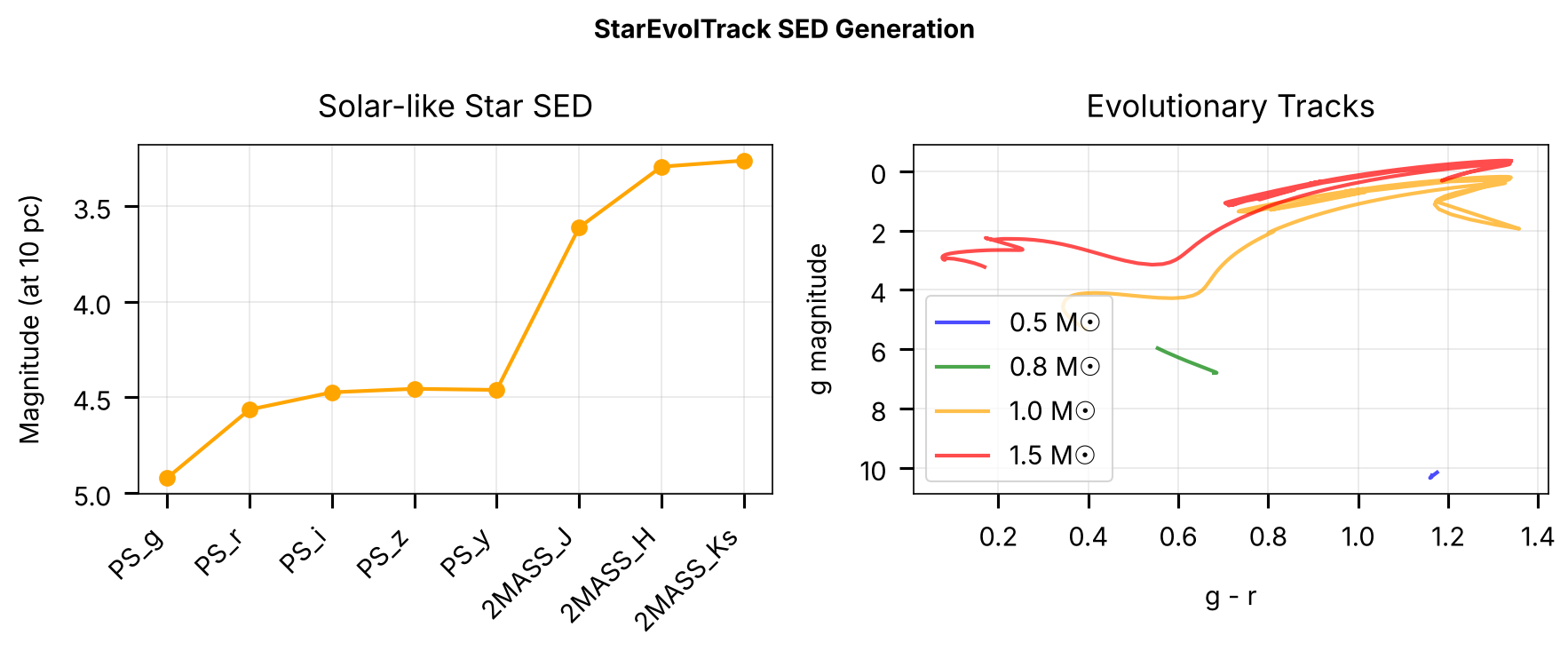
StarEvolTrack generates SEDs using neural networks for bolometric corrections. This provides on-the-fly photometry generation at any point in parameter space.
Key Features
Fast SED generation using neural networks
Support for any photometric filter system
Binary star modeling capabilities
Extinction and distance effects
from brutus.core import StarEvolTrack

# Set up filters (Pan-STARRS + 2MASS)
filt = filters.ps[:-2] + filters.tmass
print(f"Using filters: {', '.join(filt)}")

# Initialize StarEvolTrack
nnfile = find_brutus_data_file("nn_c3k.h5")
star = StarEvolTrack(tracks=tracks, nnfile=nnfile, filters=filt, verbose=False)

print("StarEvolTrack initialized with neural network bolometric corrections")
Using filters: PS_g, PS_r, PS_i, PS_z, PS_y, 2MASS_J, 2MASS_H, 2MASS_Ks
StarEvolTrack initialized with neural network bolometric corrections
# Generate SED for a solar-like star
# Generate magnitudes at 10 pc
mags, params, _ = star.get_seds(mini=1.0, feh=0.0, eep=350, dist=10.0)

print("Magnitudes at 10 pc (1 M☉, [Fe/H]=0.0, EEP=350):")
for i, (f, m) in enumerate(zip(filt, mags)):
    print(f"  {f:10s}: {m:6.3f} mag")

# Calculate some colors
g_idx = filters.ps.index('PS_g')
r_idx = filters.ps.index('PS_r')
i_idx = filters.ps.index('PS_i')

print(f"\nColors:")
print(f"  g - r = {mags[g_idx] - mags[r_idx]:.3f}")
print(f"  r - i = {mags[r_idx] - mags[i_idx]:.3f}")
Magnitudes at 10 pc (1 M☉, [Fe/H]=0.0, EEP=350):
  PS_g      :  4.921 mag
  PS_r      :  4.564 mag
  PS_i      :  4.473 mag
  PS_z      :  4.455 mag
  PS_y      :  4.461 mag
  2MASS_J   :  3.611 mag
  2MASS_H   :  3.293 mag
  2MASS_Ks  :  3.261 mag

Colors:
  g - r = 0.358
  r - i = 0.090
# Plot the SED and main sequence tracks
fig, (ax1, ax2) = plt.subplots(1, 2, figsize=(12, 5))

# Panel 1: SED in magnitudes
ax1.plot(range(len(filt)), mags, 'o-', color='orange', lw=2, ms=8)
ax1.set_xticks(range(len(filt)))
ax1.set_xticklabels(filt, rotation=45, ha='right')
ax1.set_ylabel('Magnitude (at 10 pc)')
ax1.set_title('Solar-like Star SED')
ax1.grid(True, alpha=0.3)
ax1.invert_yaxis()

# Panel 2: Color-magnitude diagram with tracks
colors = ['blue', 'green', 'orange', 'red']
masses = [0.5, 0.8, 1.0, 1.5]

for mass, color in zip(masses, colors):
    eep_range = np.linspace(202, 808, 300)  # ZAMS (202) to the TP-AGB (808)
    mags_arr = []

    for eep in eep_range:
        try:
            m, _, _ = star.get_seds(mini=mass, feh=0.0, eep=eep, dist=10.0)
            mags_arr.append(m)
        except:
            continue

    if mags_arr:
        mags_arr = np.array(mags_arr)
        g_idx = filters.ps.index('PS_g')
        r_idx = filters.ps.index('PS_r')

        ax2.plot(mags_arr[:, g_idx] - mags_arr[:, r_idx],
                 mags_arr[:, g_idx],
                 color=color, lw=2, alpha=0.7, label=f'{mass} M☉')

# Note: Lower-mass stars (< ~0.8 Msun) only evolve on timescales > age of the universe,
# so their post-MS evolution is not observable.
ax2.set_xlabel('g - r')
ax2.set_ylabel('g magnitude')
ax2.set_title('Evolutionary Tracks')
ax2.invert_yaxis()
ax2.legend(loc='lower left')
ax2.grid(True, alpha=0.3)

plt.suptitle('StarEvolTrack SED Generation', fontsize=14, fontweight='bold')
plt.tight_layout()
save_figure(fig, 'sed_generation')
plt.show()
Section 3: Stellar Evolution Along Tracks
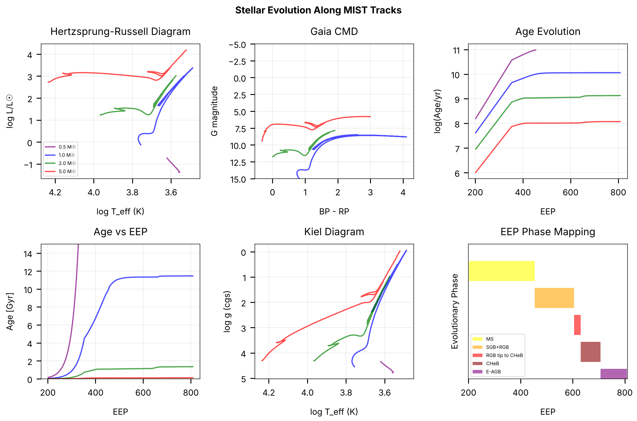
Let’s explore how stellar parameters evolve along evolutionary tracks, from the zero-age main sequence (EEP 202) to the start of the thermally pulsing asymptotic giant branch (EEP 808).
# Use Gaia filters for the HRD
filt_gaia = filters.gaia
star_gaia = StarEvolTrack(tracks=tracks, nnfile=nnfile, filters=filt_gaia, verbose=False)

# EEP ranges of the evolutionary phases, from the MIST primary EEPs
# (Dotter 2016): 202 ZAMS, 454 TAMS, 605 RGB tip, 631 zero-age core
# helium burning, 707 end of core helium burning, 808 TP-AGB
eep_phases = {
    "MS": (202, 454),
    "SGB+RGB": (454, 605),
    "RGB tip to CHeB": (605, 631),
    "CHeB": (631, 707),
    "E-AGB": (707, 808),
}

print("EEP ranges for evolutionary phases:")
for phase, (eep_min, eep_max) in eep_phases.items():
    print(f"  {phase:8s}: EEP {eep_min:3d} - {eep_max:3d}")
EEP ranges for evolutionary phases:
  MS      : EEP 202 - 454
  SGB+RGB : EEP 454 - 605
  RGB tip to CHeB: EEP 605 - 631
  CHeB    : EEP 631 - 707
  E-AGB   : EEP 707 - 808
# Create comprehensive evolution plots
fig = plt.figure(figsize=(15, 10))

# Set up subplots
ax1 = plt.subplot(2, 3, 1)  # HRD
ax2 = plt.subplot(2, 3, 2)  # CMD
ax3 = plt.subplot(2, 3, 3)  # Age evolution
ax4 = plt.subplot(2, 3, 4)  # Age in Gyr
ax5 = plt.subplot(2, 3, 5)  # Kiel diagram
ax6 = plt.subplot(2, 3, 6)  # EEP phases

# Generate tracks for different masses
masses = [0.5, 1.0, 2.0, 5.0]
colors = ['purple', 'blue', 'green', 'red']

for mass, color in zip(masses, colors):
    eep_grid = np.linspace(202, 808, 500)

    # Collect parameters along track
    params_list = []
    mags_list = []

    for eep in eep_grid:
        try:
            params_arr = tracks.get_predictions([mass, eep, 0.0, 0.0])
            params = {label: params_arr[i] for i, label in enumerate(tracks.predictions)}
            mags, _, _ = star_gaia.get_seds(mini=mass, feh=0.0, eep=eep, dist=1000.0)  # at 1 kpc
            params_list.append(params)
            mags_list.append(mags)
        except:
            continue

    if not params_list:
        continue

    # Convert to arrays
    params_arr = {key: np.array([p[key] for p in params_list]) for key in params_list[0].keys()}
    mags_arr = np.array(mags_list)

    # Panel 1: HRD
    ax1.plot(params_arr['logt'], params_arr['logl'],
             color=color, lw=2, alpha=0.7, label=f'{mass} M☉')

    # Panel 2: Gaia CMD
    bp_rp = mags_arr[:, 1] - mags_arr[:, 2]  # BP - RP
    g_mag = mags_arr[:, 0]  # G
    ax2.plot(bp_rp, g_mag, color=color, lw=2, alpha=0.7)

    # Panel 3: Age evolution
    ax3.plot(eep_grid[:len(params_list)], params_arr['loga'],
             color=color, lw=2, alpha=0.7)

    # Panel 4: Age in Gyr
    ages = 10**params_arr['loga'] / 1e9  # Convert to Gyr
    ax4.plot(eep_grid[:len(params_list)], ages,
             color=color, lw=2, alpha=0.7)

    # Panel 5: Kiel diagram
    ax5.plot(params_arr['logt'], params_arr['logg'],
             color=color, lw=2, alpha=0.7)

# Panel 6: Show evolutionary phases
phase_colors = ['yellow', 'orange', 'red', 'darkred', 'purple']
y_pos = 0.8
for (phase, (eep_min, eep_max)), color in zip(eep_phases.items(), phase_colors):
    ax6.barh(y_pos, eep_max - eep_min, left=eep_min, height=0.15,
             color=color, alpha=0.6, label=phase)
    y_pos -= 0.2

# Format all plots
ax1.set_xlabel('log T_eff (K)')
ax1.set_ylabel('log L/L☉')
ax1.set_title('Hertzsprung-Russell Diagram')
ax1.invert_xaxis()
ax1.legend(fontsize=8)
ax1.grid(True, alpha=0.3)

ax2.set_xlabel('BP - RP')
ax2.set_ylabel('G magnitude')
ax2.set_title('Gaia CMD')
ax2.invert_yaxis()
ax2.set_ylim(15, -5)
ax2.grid(True, alpha=0.3)

ax3.set_xlabel('EEP')
ax3.set_ylabel('log(Age/yr)')
ax3.set_title('Age Evolution')
ax3.grid(True, alpha=0.3)

ax4.set_xlabel('EEP')
ax4.set_ylabel('Age [Gyr]')
ax4.set_title('Age vs EEP')
ax4.set_ylim(0, 15)
ax4.grid(True, alpha=0.3)

ax5.set_xlabel('log T_eff (K)')
ax5.set_ylabel('log g (cgs)')
ax5.set_title('Kiel Diagram')
ax5.invert_xaxis()
ax5.invert_yaxis()
ax5.grid(True, alpha=0.3)

ax6.set_xlabel('EEP')
ax6.set_ylabel('Evolutionary Phase')
ax6.set_title('EEP Phase Mapping')
ax6.set_xlim(200, 810)
ax6.set_ylim(0, 1)
ax6.legend(fontsize=8, loc='lower left')
ax6.set_yticks([])

plt.suptitle('Stellar Evolution Along MIST Tracks', fontsize=16, fontweight='bold')
plt.tight_layout()
save_figure(fig, 'stellar_evolution')
plt.show()
Section 4: Metallicity Effects
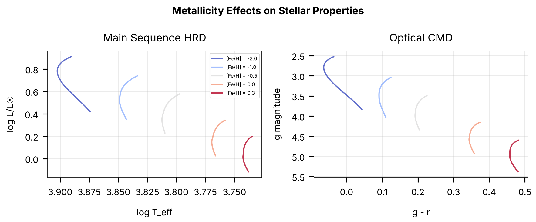
Metallicity significantly affects stellar evolution and photometry. Let’s explore how [Fe/H] changes stellar properties and colors.
# Create metallicity comparison plots
fig, axes = plt.subplots(1, 2, figsize=(12, 5))

# Different metallicities to explore
feh_values = [-2.0, -1.0, -0.5, 0.0, 0.3]
colors = plt.cm.coolwarm(np.linspace(0, 1, len(feh_values)))

# Fixed mass for comparison
test_mass = 1.0
ms_eeps = np.linspace(350, 450, 50)  # Main sequence only

for feh, color in zip(feh_values, colors):
    # Collect data
    params_list = []
    mags_list = []

    for eep in ms_eeps:
        try:
            params_arr = tracks.get_predictions([test_mass, eep, feh, 0.0])
            params = {label: params_arr[i] for i, label in enumerate(tracks.predictions)}
            mags, _, _ = star.get_seds(mini=test_mass, feh=feh, eep=eep, dist=10.0)
            params_list.append(params)
            mags_list.append(mags)
        except:
            continue

    if not params_list:
        continue

    params_arr = {key: np.array([p[key] for p in params_list]) for key in params_list[0].keys()}
    mags_arr = np.array(mags_list)

    # Panel 1: HRD
    axes[0].plot(params_arr['logt'], params_arr['logl'],
                    color=color, lw=2, alpha=0.8, label=f'[Fe/H] = {feh:.1f}')

    # Panel 2: Optical CMD
    g_idx = filters.ps.index('PS_g')
    r_idx = filters.ps.index('PS_r')
    axes[1].plot(mags_arr[:, g_idx] - mags_arr[:, r_idx], mags_arr[:, g_idx],
                    color=color, lw=2, alpha=0.8)

# Format plots
axes[0].set_xlabel('log T_eff')
axes[0].set_ylabel('log L/L☉')
axes[0].set_title('Main Sequence HRD')
axes[0].invert_xaxis()
axes[0].legend(fontsize=8)
axes[0].grid(True, alpha=0.3)

axes[1].set_xlabel('g - r')
axes[1].set_ylabel('g magnitude')
axes[1].set_title('Optical CMD')
axes[1].invert_yaxis()
axes[1].grid(True, alpha=0.3)

plt.suptitle('Metallicity Effects on Stellar Properties', fontsize=16, fontweight='bold')
plt.tight_layout()
save_figure(fig, 'metallicity_effects')
plt.show()
Section 5: Binary Star Modeling
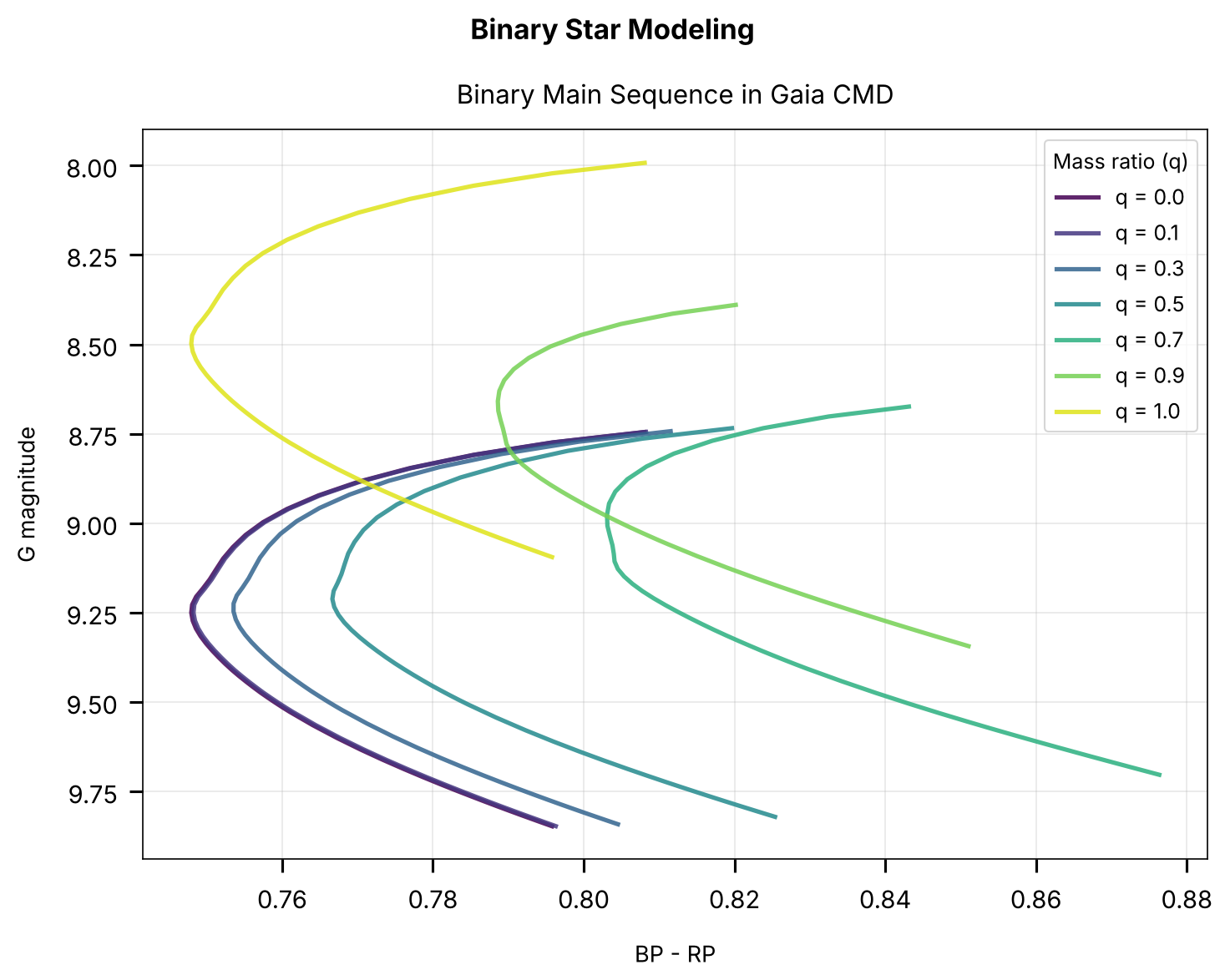
Unresolved binaries significantly affect observed photometry. StarEvolTrack can model binary systems using the secondary mass fraction (SMF).
Binary Parameters
SMF (Secondary Mass Fraction): q = M₂/M₁ where M₁ is the primary mass
Equal-age assumption: Both stars have the same age and metallicity
Combined light: Total flux is the sum of both components
# Set up for binary modeling
filt_binary = filters.gaia + filters.ps[:3]  # Gaia + PS optical
star_binary = StarEvolTrack(tracks=tracks, nnfile=nnfile, filters=filt_binary, verbose=False)

# Binary parameters to explore
primary_mass = 1.0  # Solar mass primary
smf_values = [0.0, 0.3, 0.5, 0.7, 1.0]  # Single to equal-mass binary
colors_smf = ['blue', 'cyan', 'green', 'orange', 'red']

print("Binary mass ratios to explore:")
for smf in smf_values:
    secondary_mass = primary_mass * smf
    print(f"  q = {smf:.1f}: M₁ = {primary_mass:.1f} M☉, M₂ = {secondary_mass:.1f} M☉")
Binary mass ratios to explore:
  q = 0.0: M₁ = 1.0 M☉, M₂ = 0.0 M☉
  q = 0.3: M₁ = 1.0 M☉, M₂ = 0.3 M☉
  q = 0.5: M₁ = 1.0 M☉, M₂ = 0.5 M☉
  q = 0.7: M₁ = 1.0 M☉, M₂ = 0.7 M☉
  q = 1.0: M₁ = 1.0 M☉, M₂ = 1.0 M☉
# Create binary main sequence plot with multiple mass ratios
fig, ax = plt.subplots(figsize=(10, 8))

eep_range = np.linspace(300, 454, 50)

smf_values_plot = [0.0, 0.1, 0.3, 0.5, 0.7, 0.9, 1.0]
colors_plot = plt.cm.viridis(np.linspace(0, 0.95, len(smf_values_plot)))

for smf, color in zip(smf_values_plot, colors_plot):
    g_mags = []
    bp_rp_colors = []

    for eep in eep_range:
        try:
            mags, _, _ = star_binary.get_seds(
                mini=1.0, feh=0.0, eep=eep, smf=smf, dist=100.0
            )
            g_mags.append(mags[0])
            bp_rp_colors.append(mags[1] - mags[2])
        except:
            continue

    if g_mags:
        ax.plot(bp_rp_colors, g_mags, color=color, lw=2.5,
                alpha=0.85, label=f'q = {smf:.1f}')

ax.set_xlabel('BP - RP', fontsize=13)
ax.set_ylabel('G magnitude', fontsize=13)
ax.set_title('Binary Main Sequence in Gaia CMD', fontsize=15)
ax.invert_yaxis()
ax.legend(fontsize=12, title='Mass ratio (q)', title_fontsize=12)
ax.grid(True, alpha=0.3)

plt.suptitle('Binary Star Modeling', fontsize=16, fontweight='bold')
plt.tight_layout()
save_figure(fig, 'binary_modeling')
plt.show()
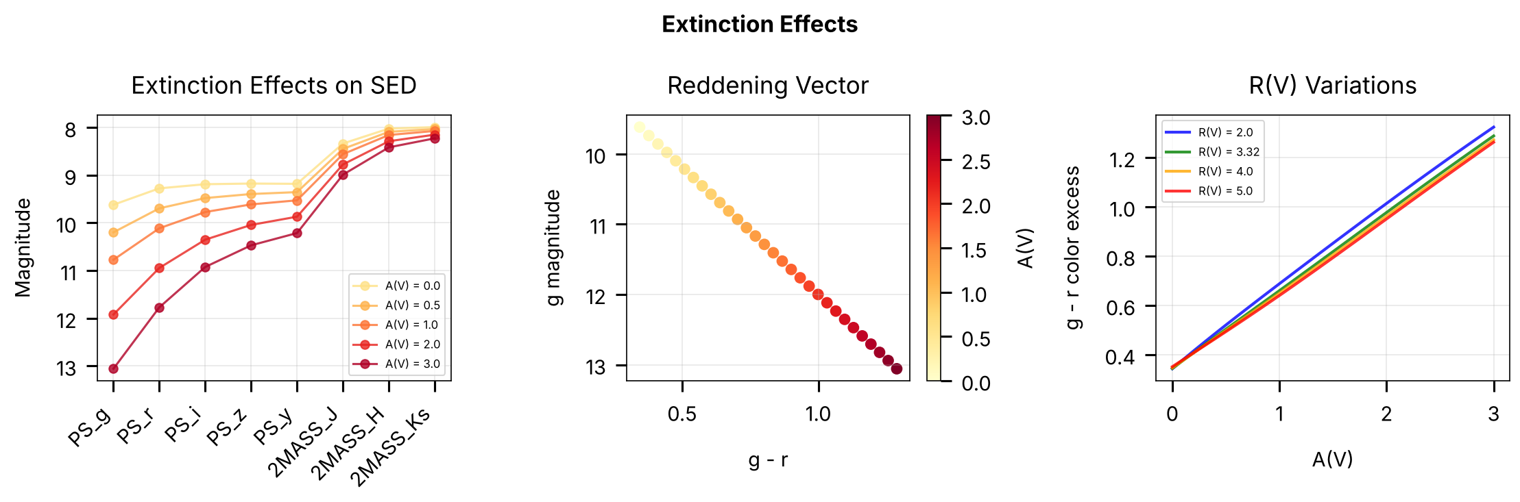
Section 6: Extinction and Distance Effects
Interstellar extinction and distance are critical for interpreting photometry. Let’s explore how these affect observed SEDs and colors.
Key Parameters
A(V): Visual extinction in magnitudes
R(V): Total-to-selective extinction ratio (typically 3.32)
Distance modulus: μ = 5 log₁₀(d/10) where d is in parsecs
# Create extinction plots
fig, axes = plt.subplots(1, 3, figsize=(15, 5))

# Test star parameters
mini, feh, eep = 1.0, 0.0, 400

# Panel 1: Extinction effects on SED
ax = axes[0]
av_values = [0.0, 0.5, 1.0, 2.0, 3.0]
colors_av = plt.cm.YlOrRd(np.linspace(0.2, 0.9, len(av_values)))

for av, color in zip(av_values, colors_av):
    mags, _, _ = star.get_seds(
        mini=mini, feh=feh, eep=eep, av=av, rv=3.32, dist=100.0
    )
    ax.plot(range(len(filt)), mags, 'o-', color=color,
            alpha=0.8, label=f'A(V) = {av}')

ax.set_xticks(range(len(filt)))
ax.set_xticklabels(filt, rotation=45, ha='right')
ax.set_ylabel('Magnitude')
ax.set_title('Extinction Effects on SED')
ax.legend(fontsize=8)
ax.invert_yaxis()
ax.grid(True, alpha=0.3)

# Panel 2: Reddening vector in CMD
ax = axes[1]
g_idx = filters.ps.index('PS_g')
r_idx = filters.ps.index('PS_r')

av_range = np.linspace(0, 3, 30)
g_mags, colors = [], []

for av in av_range:
    mags, _, _ = star.get_seds(
        mini=mini, feh=feh, eep=eep, av=av, rv=3.32, dist=100.0
    )
    g_mags.append(mags[g_idx])
    colors.append(mags[g_idx] - mags[r_idx])

scatter = ax.scatter(colors, g_mags, c=av_range, cmap='YlOrRd', s=50)
plt.colorbar(scatter, ax=ax, label='A(V)')
ax.set_xlabel('g - r')
ax.set_ylabel('g magnitude')
ax.set_title('Reddening Vector')
ax.invert_yaxis()
ax.grid(True, alpha=0.3)

# Panel 3: R(V) variations
ax = axes[2]
rv_values = [2.0, 3.32, 4.0, 5.0]
colors_rv = ['blue', 'green', 'orange', 'red']

for rv, color in zip(rv_values, colors_rv):
    colors_temp = []
    for av in av_range:
        mags, _, _ = star.get_seds(
            mini=mini, feh=feh, eep=eep, av=av, rv=rv, dist=100.0
        )
        colors_temp.append(mags[g_idx] - mags[r_idx])
    ax.plot(av_range, colors_temp, color=color, lw=2,
            alpha=0.8, label=f'R(V) = {rv}')

ax.set_xlabel('A(V)')
ax.set_ylabel('g - r color excess')
ax.set_title('R(V) Variations')
ax.legend(fontsize=8)
ax.grid(True, alpha=0.3)

plt.suptitle('Extinction Effects', fontsize=16, fontweight='bold')
plt.tight_layout()
save_figure(fig, 'extinction_distance')
plt.show()
Section 7: FastNN and FastNNPredictor
FastNNPredictor (and its base class FastNN) evaluates the bolometric-correction neural network directly from atmospheric and physical parameters without interpolating evolutionary tracks:
StarEvolTrack: maps evolutionary inputs (mini,eep,feh,afe) to surface parameters (logt,logg,feh_surf,logl,afe_surf) viaEEPTracks, then evaluatesFastNNPredictor.FastNNPredictor: accepts (logt,logg,feh_surf,logl,afe,av,rv,dist) directly and returns apparent magnitudes.
When given the surface parameters resolved by StarEvolTrack, FastNNPredictor.sed() returns identical magnitudes.
# Initialize FastNNPredictor with the same filters used earlier
try:
    from brutus.core import FastNNPredictor

    fastnn = FastNNPredictor(filters=filt, nnfile=str(nnfile), verbose=False)
    print(f"FastNNPredictor initialized with {fastnn.NFILT} filters: {', '.join(filt)}")

    # Predict magnitudes for a solar-like star at 1 kpc with mild extinction
    fastnn_mags = fastnn.sed(
        logt=3.76, logg=4.44, feh_surf=0.0, logl=0.0, afe=0.0,
        av=0.1, rv=3.3, dist=1000.0
    )

    print(f"\nFastNNPredictor magnitudes (logt=3.76, logg=4.44, feh=0.0, logl=0.0,")
    print(f"                            afe=0.0, av=0.1, rv=3.3, dist=1000 pc):\n")
    for f, m in zip(filt, fastnn_mags):
        print(f"  {f:10s}: {m:7.3f} mag")

    fastnn_available = True

except Exception as e:
    print(f"FastNNPredictor not available (data file missing?): {e}")
    print("Skipping FastNN examples. Run the download cell at the top to fetch data files.")
    fastnn_available = False
FastNNPredictor initialized with 8 filters: PS_g, PS_r, PS_i, PS_z, PS_y, 2MASS_J, 2MASS_H, 2MASS_Ks

FastNNPredictor magnitudes (logt=3.76, logg=4.44, feh=0.0, logl=0.0,
                            afe=0.0, av=0.1, rv=3.3, dist=1000 pc):

  PS_g      :  15.122 mag
  PS_r      :  14.711 mag
  PS_i      :  14.585 mag
  PS_z      :  14.546 mag
  PS_y      :  14.539 mag
  2MASS_J   :  13.669 mag
  2MASS_H   :  13.329 mag
  2MASS_Ks  :  13.290 mag
# Compare FastNNPredictor vs StarEvolTrack predictions
# StarEvolTrack resolves (mini, eep, feh) -> physical params -> magnitudes.
# We can extract the intermediate physical params and feed them directly
# to FastNNPredictor to verify the two paths give identical results.

if fastnn_available:
    # Use StarEvolTrack to get magnitudes AND the resolved physical parameters
    # for a 1 Msun main-sequence star (EEP 350) at 1 kpc with mild extinction
    set_mags, set_params, _ = star.get_seds(
        mini=1.0, feh=0.0, eep=350, av=0.1, rv=3.3, dist=1000.0
    )

    # Now call FastNNPredictor with the same physical parameters
    fastnn_compare = fastnn.sed(
        logt=set_params['logt'],
        logg=set_params['logg'],
        feh_surf=set_params['feh_surf'],
        logl=set_params['logl'],
        afe=set_params['afe_surf'],
        av=0.1,
        rv=3.3,
        dist=1000.0,
    )

    # Print comparison table
    print("Comparison: StarEvolTrack vs FastNNPredictor")
    print("(Using identical physical params from a 1 Msun main-sequence star)\n")
    print(f"Resolved params: logt={set_params['logt']:.4f}, logg={set_params['logg']:.4f}, "
          f"feh_surf={set_params['feh_surf']:.4f}, logl={set_params['logl']:.4f}, "
          f"afe_surf={set_params['afe_surf']:.4f}\n")
    print(f"{'Filter':10s}  {'StarEvolTrack':>14s}  {'FastNNPredictor':>15s}  {'Difference':>10s}")
    print("-" * 55)
    for f, m_set, m_fnn in zip(filt, set_mags, fastnn_compare):
        diff = m_fnn - m_set
        print(f"{f:10s}  {m_set:14.4f}  {m_fnn:15.4f}  {diff:10.6f}")

    # Verify they match (should be identical since same NN is used)
    max_diff = np.max(np.abs(fastnn_compare - set_mags))
    print(f"\nMax absolute difference: {max_diff:.2e} mag")
    assert max_diff < 0.1, f"Predictions differ by more than 0.1 mag (max diff: {max_diff:.4f})"
    print("Assertion passed: all differences < 0.1 mag")
else:
    print("Skipping comparison (FastNNPredictor not available).")
Comparison: StarEvolTrack vs FastNNPredictor
(Using identical physical params from a 1 Msun main-sequence star)

Resolved params: logt=3.7662, logg=4.4321, feh_surf=-0.0143, logl=0.0256, afe_surf=0.0000

Filter       StarEvolTrack  FastNNPredictor  Difference
-------------------------------------------------------
PS_g               15.0376          15.0376    0.000000
PS_r               14.6473          14.6473    0.000000
PS_i               14.5309          14.5309    0.000000
PS_z               14.4992          14.4992    0.000000
PS_y               14.4958          14.4958    0.000000
2MASS_J            13.6341          13.6341    0.000000
2MASS_H            13.3069          13.3069    0.000000
2MASS_Ks           13.2696          13.2696    0.000000

Max absolute difference: 0.00e+00 mag
Assertion passed: all differences < 0.1 mag
Summary and Key Takeaways
This tutorial has covered the fundamental components for modeling individual stars in brutus:
Key Classes
EEPTracks: Provides stellar parameter predictions along evolutionary tracks
Interpolates MIST stellar evolution models
Returns physical parameters (Teff, log g, luminosity, age)
Covers full evolutionary phases from pre-MS to post-AGB
StarEvolTrack: Generates SEDs using neural networks
Fast bolometric corrections via neural networks
Supports any photometric filter system
Includes binary star modeling (SMF parameter)
Handles extinction (A(V), R(V)) and distance
FastNNPredictor: Lightweight SED prediction from physical parameters
Skips evolutionary track interpolation entirely
Takes physical parameters (Teff, log g, [Fe/H], L, Av, Rv) directly
Produces identical results to StarEvolTrack when given matching parameters
Useful when stellar parameters are already known
Physical Effects
Metallicity: Affects temperature, color, and evolutionary timescales
Binaries: Create sequences above the main sequence
Extinction: Reddens and dims stellar light
Distance: Determines apparent magnitude via distance modulus
Next Steps
Tutorial 2: Stellar Population Models (Isochrones and StellarPop)
Tutorial 3: Grid Generation and Performance Optimization
Tutorial 4: Galactic Priors and Population Synthesis
Tutorial 5: Fitting Individual Sources with BruteForce