Tutorial 4: Galactic Priors and Models

brutus.priors implements the 3D Galactic density, 3D dust extinction, astrometric parallax, initial mass function, metallicity, and age-metallicity priors used during Bayesian stellar inference.

Topics Covered

1. Galactic structure priors (thin disk, thick disk, halo)

2. 3D dust priors with Bayestar

3. Distance and parallax priors

4. Prior factorization and combination

5. Metallicity and age-metallicity priors

Prerequisites

The setup cell below checks the data files this tutorial needs; Tutorial 00 shows how to download them.

# Optional: Download required data files (only needed if not already cached)
# Uncomment the lines below to download them.

# from brutus.data import fetch_dustmaps
# fetch_dustmaps()  # optional

# Imports and setup
import numpy as np
import matplotlib.pyplot as plt
from pathlib import Path
import warnings
warnings.filterwarnings('ignore')

from tutorial_utils import (
    setup_tutorial,
    print_saved_files,
    find_brutus_data_file,
    save_figure as _save_fig,
    print_section,
)

info = setup_tutorial(4, title="Tutorial 04: Galactic Priors and Models")


def save_figure(fig, name):
    """Save figure to this tutorial's plot directory."""
    _save_fig(fig, 4, name)

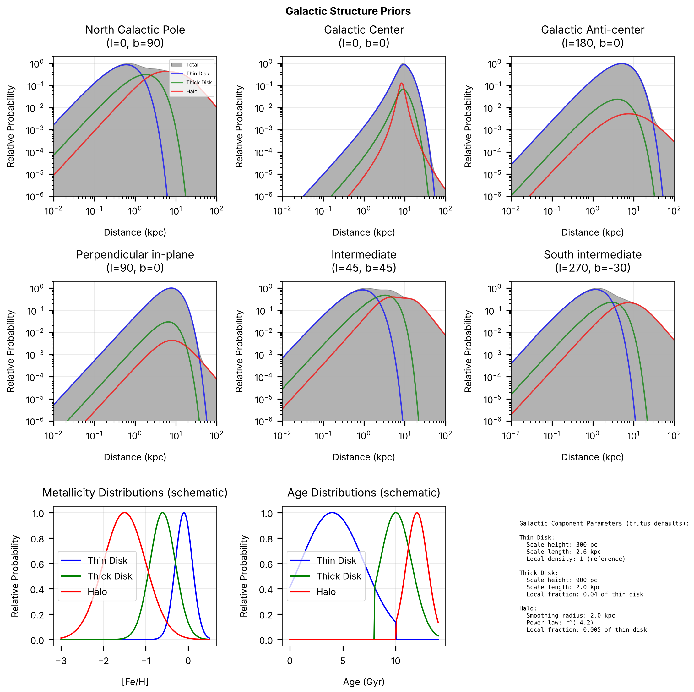
Section 1: Galactic Structure - 3D Density Models

The Galaxy has distinct structural components with different spatial distributions, ages, and metallicities.

Components

• Thin Disk: Scale height ~300 pc, young/metal-rich stars

• Thick Disk: Scale height ~900 pc, old/metal-poor stars

• Halo: Power-law profile, very old/metal-poor stars

Each component dominates at different Galactic latitudes and distances.

from brutus.priors.galactic import logp_galactic_structure, logn_disk, logn_halo

# Create Galactic structure visualization  
fig, axes = plt.subplots(3, 3, figsize=(15, 15))

# Define sightlines
sightlines = [
    (0, 90, 'North Galactic Pole'),
    (0, 0, 'Galactic Center'),
    (180, 0, 'Galactic Anti-center'),
    (90, 0, 'Perpendicular in-plane'),
    (45, 45, 'Intermediate'),
    (270, -30, 'South intermediate')
]

# Distance grid
distances = np.logspace(-2, 2, 200)  # 0.01 to 100 kpc

for idx, (l, b, title) in enumerate(sightlines[:6]):
    ax = axes[idx // 3, idx % 3]
    
    coord = np.array([l, b])
    
    # Get prior
    with warnings.catch_warnings():
        warnings.simplefilter("ignore")
        lnp = logp_galactic_structure(distances, coord)
    
    # Convert to cylindrical coordinates for component visualization
    from astropy.coordinates import SkyCoord, CylindricalRepresentation as CylRep
    import astropy.units as units
    
    ell = np.full_like(distances, l)
    b_arr = np.full_like(distances, b)
    coords = SkyCoord(l=ell * units.deg, b=b_arr * units.deg,
                     distance=distances * units.kpc, frame='galactic')
    coords_cyl = coords.galactocentric.cartesian.represent_as(CylRep)
    R, Z = coords_cyl.rho.value, coords_cyl.z.value
    
    # Compute individual components
    vol_factor = 2 * np.log(distances + 1e-300)
    lnp_thin = logn_disk(R, Z, R_scale=2.6, Z_scale=0.3) + vol_factor
    lnp_thick = logn_disk(R, Z, R_scale=2.0, Z_scale=0.9) + vol_factor + np.log(0.04)
    lnp_halo = logn_halo(R, Z) + vol_factor + np.log(0.005)
    
    # Convert to probabilities
    p_total = np.exp(lnp - np.max(lnp))
    p_thin = np.exp(lnp_thin - np.max(lnp))
    p_thick = np.exp(lnp_thick - np.max(lnp))
    p_halo = np.exp(lnp_halo - np.max(lnp))
    
    # Plot components
    ax.fill_between(distances, p_total, alpha=0.3, color='black', label='Total')
    ax.loglog(distances, p_thin, 'b-', lw=2, alpha=0.7, label='Thin Disk')
    ax.loglog(distances, p_thick, 'g-', lw=2, alpha=0.7, label='Thick Disk')
    ax.loglog(distances, p_halo, 'r-', lw=2, alpha=0.7, label='Halo')
    
    ax.set_xlabel('Distance (kpc)')
    ax.set_ylabel('Relative Probability')
    ax.set_title(f'{title}\n(l={l}, b={b})')
    ax.set_xlim(0.01, 100)
    ax.set_ylim(1e-6, 2)
    ax.grid(True, alpha=0.3)
    
    if idx == 0:
        ax.legend(fontsize=8, loc='upper right')

# Panel 7: Metallicity distributions
ax = axes[2, 0]

feh_range = np.linspace(-3, 0.5, 200)

# Component metallicity distributions (schematic)
thin_feh = np.exp(-(feh_range + 0.1)**2 / (2 * 0.2**2))
thick_feh = np.exp(-(feh_range + 0.6)**2 / (2 * 0.3**2))
halo_feh = np.exp(-(feh_range + 1.5)**2 / (2 * 0.5**2))

ax.plot(feh_range, thin_feh/thin_feh.max(), 'b-', lw=2, label='Thin Disk')
ax.plot(feh_range, thick_feh/thick_feh.max(), 'g-', lw=2, label='Thick Disk')
ax.plot(feh_range, halo_feh/halo_feh.max(), 'r-', lw=2, label='Halo')

ax.set_xlabel('[Fe/H]')
ax.set_ylabel('Relative Probability')
ax.set_title('Metallicity Distributions (schematic)')
ax.legend()
ax.grid(True, alpha=0.3)

# Panel 8: Age distributions
ax = axes[2, 1]

age_range = np.linspace(0, 14, 200)  # Gyr

thin_age = np.exp(-(age_range - 4)**2 / (2 * 3**2)) * (age_range < 10)
thick_age = np.exp(-(age_range - 10)**2 / (2 * 1.5**2)) * (age_range > 8)
halo_age = np.exp(-(age_range - 12)**2 / (2 * 1**2)) * (age_range > 10)

ax.plot(age_range, thin_age/thin_age.max(), 'b-', lw=2, label='Thin Disk')
ax.plot(age_range, thick_age/thick_age.max(), 'g-', lw=2, label='Thick Disk')
ax.plot(age_range, halo_age/halo_age.max(), 'r-', lw=2, label='Halo')

ax.set_xlabel('Age (Gyr)')
ax.set_ylabel('Relative Probability')
ax.set_title('Age Distributions (schematic)')
ax.legend()
ax.grid(True, alpha=0.3)

# Panel 9: Parameters text
ax = axes[2, 2]
ax.axis('off')

components_info = """
Galactic Component Parameters (brutus defaults):

Thin Disk:
  Scale height: 300 pc
  Scale length: 2.6 kpc
  Local density: 1 (reference)

Thick Disk:
  Scale height: 900 pc
  Scale length: 2.0 kpc
  Local fraction: 0.04 of thin disk

Halo:
  Smoothing radius: 2.0 kpc
  Power law: r^(-4.2)
  Local fraction: 0.005 of thin disk
"""

ax.text(0.05, 0.95, components_info, transform=ax.transAxes,
       fontsize=9, va='top', family='monospace')

plt.suptitle('Galactic Structure Priors', fontsize=16, fontweight='bold')
save_figure(fig, 'galactic_structure')
plt.show()

Section 2: 3D Dust Extinction

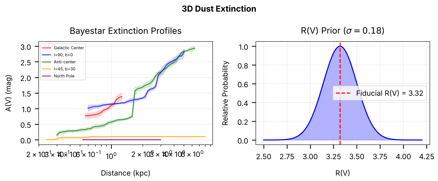
The Bayestar class in brutus.dust provides distance-resolved extinction estimates. For any Galactic sightline, it returns A(V) mean and standard deviation as a function of distance, based on Pan-STARRS and 2MASS photometry.

Key properties:

• 120 distance bins from ~0.06 to ~60 kpc at ~7 arcmin HEALPix resolution

• A(V) uncertainty grows with distance

• Extinction concentrated near the Galactic plane

• Returns uniform prior for sightlines outside map coverage

• By default, queries honor the map’s per-pixel reliability metadata, returning NaN for distance bins outside a pixel’s reliable distance range and for pixels whose fits did not converge (pass Bayestar(..., apply_reliability_mask=False) for the raw, unmasked profiles)

The logp_extinction function wraps Bayestar queries to provide a Gaussian log-prior on A(V) at a given distance and sky position, truncated and renormalized over the fitted A(V) range (avlim).

Coverage limitations: Bayestar is based on Pan-STARRS photometry and has no coverage in the southern sky below declination ~ -30 degrees. Coverage is also incomplete near the Galactic center due to extreme crowding and extinction. For sightlines outside the map footprint (and, with the default reliability masking, for distance bins the map flags as unreliable), logp_extinction returns a uniform (uninformative) prior normalized over avlim like the Gaussian. Where the map is informative, a 0.2 mag systematic scatter (scatter=0.2) is added in quadrature to the map’s A(V) spread.

# 3D Dust extinction demonstration using the Bayestar dust map
#
# The Bayestar class provides distance-resolved extinction profiles:
#   distances, av_mean, av_std = dustmap.query(coord)
# Each sightline returns A(V) as a function of distance.

# Try to load the real Bayestar dust map
dustmap = None
try:
    from brutus.dust import Bayestar
    dustfile = find_brutus_data_file('bayestar2019_v1.h5')
    dustmap = Bayestar(dustfile=dustfile)
    print(f"Loaded Bayestar dust map from {Path(dustfile).name}")
    dust_available = True
except (FileNotFoundError, ImportError) as e:
    print(f"Bayestar dust map not available: {e}")
    print("  Using synthetic data for illustration.")
    dust_available = False

fig, axes = plt.subplots(1, 2, figsize=(12, 5))

# Define sightlines for dust queries
sightlines_dust = [
    (0, 0, 'Galactic Center', 'red'),
    (90, 0, 'l=90, b=0', 'blue'),
    (180, 0, 'Anti-center', 'green'),
    (45, 30, 'l=45, b=30', 'orange'),
    (0, 90, 'North Pole', 'purple'),
]

# Panel 1: A(V) vs distance for different sightlines
ax = axes[0]

if dust_available:
    from astropy.coordinates import SkyCoord
    import astropy.units as units

    for l, b, label, color in sightlines_dust:
        coord = SkyCoord(l=l * units.deg, b=b * units.deg, frame='galactic')
        dists, av_mean, av_std = dustmap.query(coord)

        finite = np.isfinite(av_mean)
        if np.any(finite):
            ax.plot(dists[finite], av_mean[finite], color=color, lw=2,
                    alpha=0.7, label=label)
            ax.fill_between(dists[finite],
                            (av_mean - av_std)[finite],
                            (av_mean + av_std)[finite],
                            alpha=0.15, color=color)
            print(f"  (l={l:3d}, b={b:+3d}): max A(V) = {np.nanmax(av_mean):.2f}")

    ax.set_xlabel('Distance (kpc)')
    ax.set_ylabel('A(V) (mag)')
    ax.set_title('Bayestar Extinction Profiles')
    ax.set_xscale('log')
    ax.legend(fontsize=8)
    ax.grid(True, alpha=0.3)
else:
    # Synthetic fallback
    distances_synth = np.logspace(-1, 1.5, 100)
    for l, b, label, color in sightlines_dust:
        scale = np.exp(-abs(b) / 15.0)
        av_synth = 1.5 * scale * (1 - np.exp(-distances_synth / 2.0))
        ax.plot(distances_synth, av_synth, color=color, lw=2, alpha=0.7, label=label)
    ax.set_xlabel('Distance (kpc)')
    ax.set_ylabel('A(V) (mag)')
    ax.set_title('Extinction vs Distance (synthetic)')
    ax.set_xscale('log')
    ax.legend(fontsize=8)
    ax.grid(True, alpha=0.3)

# Panel 2: R(V) prior
ax = axes[1]

rv_values = np.linspace(2.5, 4.2, 200)
rv_prob = np.exp(-(rv_values - 3.32)**2 / (2 * 0.18**2))
ax.plot(rv_values, rv_prob / rv_prob.max(), 'b-', lw=2)
ax.axvline(3.32, color='red', ls='--', lw=2, label='Fiducial R(V) = 3.32')
ax.fill_between(rv_values, rv_prob / rv_prob.max(), alpha=0.3, color='blue')

ax.set_xlabel('R(V)')
ax.set_ylabel('Relative Probability')
ax.set_title(r'R(V) Prior ($\sigma = 0.18$)')
ax.legend()
ax.grid(True, alpha=0.3)

plt.suptitle('3D Dust Extinction', fontsize=16, fontweight='bold')
plt.tight_layout()
save_figure(fig, 'dust_extinction')
plt.show()

Loaded Bayestar dust map from bayestar2019_v1.h5
  (l=  0, b= +0): max A(V) = 1.38
  (l= 90, b= +0): max A(V) = 2.81
  (l=180, b= +0): max A(V) = 2.93
  (l= 45, b=+30): max A(V) = 0.10
  (l=  0, b=+90): max A(V) = 0.01

Section 3: Parallax and Distance Priors

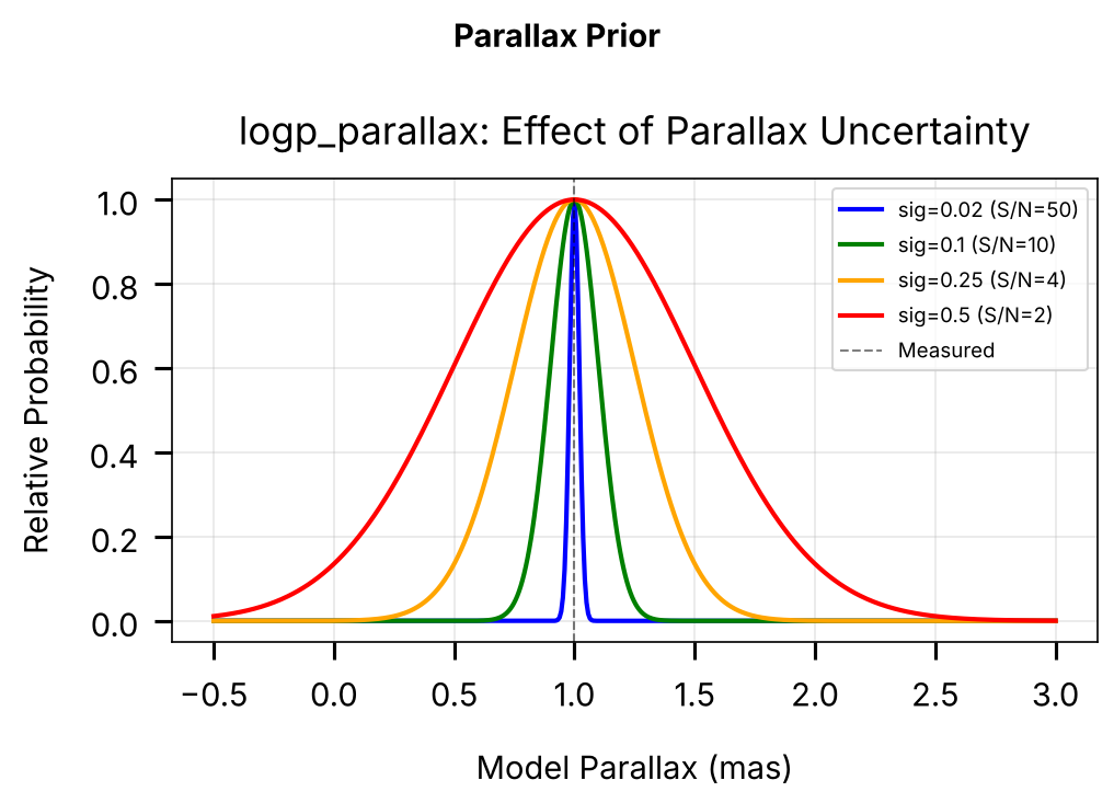
Parallax measurements from Gaia constrain stellar distances. The logp_parallax function provides a Gaussian log-prior on the model parallax given an observed parallax and its uncertainty.

Key concepts:

• Non-linear transformation: d = 1/pi leads to asymmetric distance uncertainties

• Lutz-Kelker bias: Volume effects bias distance estimates outward at low signal-to-noise

from brutus.priors.astrometric import logp_parallax

# Parallax prior visualization: effect of measurement uncertainty
fig, ax = plt.subplots(figsize=(7, 5))

parallax_grid = np.linspace(-0.5, 3.0, 500)
p_meas = 1.0

for sigma, color, label in [(0.02, 'blue', 'sig=0.02 (S/N=50)'),
                              (0.1, 'green', 'sig=0.1 (S/N=10)'),
                              (0.25, 'orange', 'sig=0.25 (S/N=4)'),
                              (0.5, 'red', 'sig=0.5 (S/N=2)')]:
    lnp = logp_parallax(parallax_grid, p_meas, sigma)
    p = np.exp(lnp - np.max(lnp))
    ax.plot(parallax_grid, p, lw=2, color=color, label=label)

ax.axvline(p_meas, color='black', ls='--', lw=1, alpha=0.5, label='Measured')
ax.set_xlabel('Model Parallax (mas)')
ax.set_ylabel('Relative Probability')
ax.set_title('logp_parallax: Effect of Parallax Uncertainty')
ax.legend(fontsize=9)
ax.grid(True, alpha=0.3)

plt.suptitle('Parallax Prior', fontsize=14, fontweight='bold')
fig.tight_layout()
save_figure(fig, 'parallax_distance')
plt.show()

Section 4: Prior Factorization and Combination

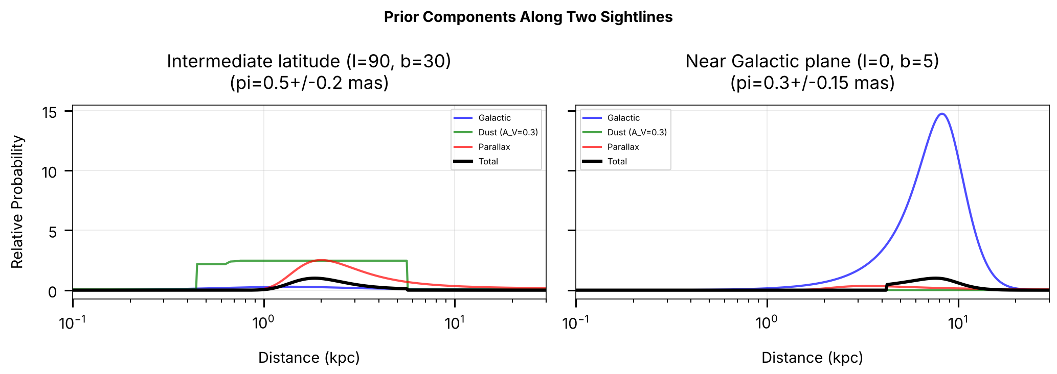
The complete prior in brutus combines all components multiplicatively, with proper factorization based on conditional independence.

Prior Factorization

The full prior can be written as:

P(θ) = P(M) × P(d,Z,τ|l,b) × P(A_V|d,l,b) × P(π_obs|d)

Where:

• P(M): IMF prior on stellar mass

• P(d,Z,τ|l,b): Galactic structure prior (distance, metallicity, age given position)

• P(A_V|d,l,b): 3D dust prior (extinction given distance and position)

• P(π_obs|d): Parallax likelihood (observed parallax given true distance)

# Demonstrate prior combination using real brutus prior functions.
# The `dustmap` variable was loaded in the Bayestar cell above.

from brutus.priors.extinction import logp_extinction

# Create combined prior visualization: two sightlines
fig, axes = plt.subplots(1, 2, figsize=(14, 5), sharey=True)

# Define two sightlines for comparison
sightline_configs = [
    (90, 30, 0.5, 0.2, 'Intermediate latitude (l=90, b=30)'),
    (0, 5, 0.3, 0.15, 'Near Galactic plane (l=0, b=5)'),
]

distances = np.logspace(-1, 1.5, 500)

for ax, (l, b, obs_parallax, sigma_parallax, title) in zip(axes, sightline_configs):
    coord = np.array([l, b])

    # Compute individual prior components using real brutus functions
    with warnings.catch_warnings():
        warnings.simplefilter("ignore")
        lnp_gal = logp_galactic_structure(distances, coord)

    # 3D dust extinction prior
    av_test = 0.3
    if dust_available and dustmap is not None:
        lnp_dust = logp_extinction(
            np.full_like(distances, av_test), dustmap, coord, distance=distances
        )
        dust_label = f'Dust (A_V={av_test})'
    else:
        av_expected = 0.3 * (1 - np.exp(-distances / 3.0))
        lnp_dust = -0.5 * ((av_test - av_expected) / 0.2)**2
        dust_label = f'Dust (A_V={av_test}, synthetic)'

    # Parallax constraint
    true_parallax = 1.0 / distances
    lnp_par = logp_parallax(true_parallax, obs_parallax, sigma_parallax)

    # Total prior (sum in log-space = product in linear space)
    lnp_total = lnp_gal + lnp_dust + lnp_par

    # Normalize all components relative to the SAME reference (the total's max)
    # so that p_total = p_gal * p_dust * p_parallax visually
    ref = np.max(lnp_total)
    p_gal = np.exp(lnp_gal - ref)
    p_dust = np.exp(lnp_dust - ref)
    p_parallax = np.exp(lnp_par - ref)
    p_total = np.exp(lnp_total - ref)

    ax.plot(distances, p_gal, 'b-', lw=2, alpha=0.7, label='Galactic')
    ax.plot(distances, p_dust, 'g-', lw=2, alpha=0.7, label=dust_label)
    ax.plot(distances, p_parallax, 'r-', lw=2, alpha=0.7, label='Parallax')
    ax.plot(distances, p_total, 'k-', lw=3, label='Total')

    ax.set_xlabel('Distance (kpc)')
    ax.set_title(f'{title}\n(pi={obs_parallax}+/-{sigma_parallax} mas)')
    ax.set_xscale('log')
    ax.set_xlim(0.1, 30)
    ax.legend(fontsize=8)
    ax.grid(True, alpha=0.3)

axes[0].set_ylabel('Relative Probability')

plt.suptitle('Prior Components Along Two Sightlines', fontsize=14, fontweight='bold')
plt.tight_layout()
save_figure(fig, 'prior_combination')
plt.show()

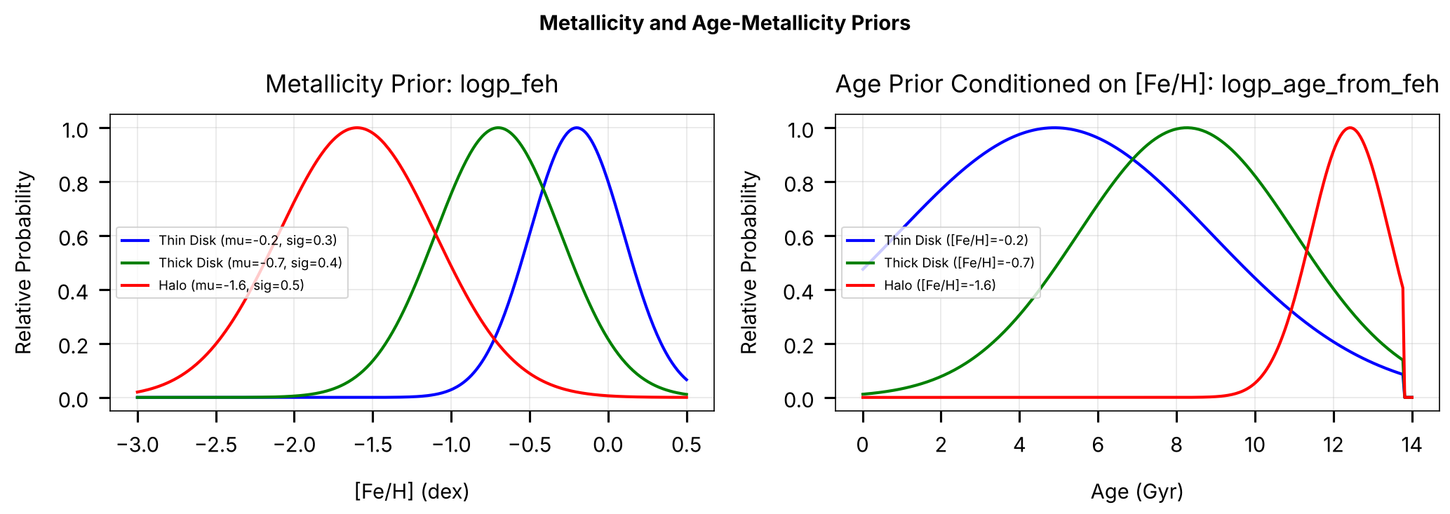
Section 5: Metallicity and Age-Metallicity Priors

Beyond Galactic structure, brutus provides priors on stellar metallicity and an age-metallicity relation that encodes the observed correlation between stellar age and chemical enrichment.

Metallicity Prior: logp_feh

The metallicity prior is a simple Gaussian parameterized by a mean and dispersion, with typical values for each Galactic component:

• Thin disk: feh_mean = -0.2, feh_sigma = 0.3

• Thick disk: feh_mean = -0.7, feh_sigma = 0.4

• Halo: feh_mean = -1.6, feh_sigma = 0.5

Age-Metallicity Relation: logp_age_from_feh

The age prior is conditioned on metallicity through a logistic age-metallicity relation: metal-poor stars are preferentially older, while metal-rich stars are preferentially younger. The mean age and its dispersion are both functions of feh_mean, with ages drawn from a truncated normal distribution bounded by physically reasonable limits.

from brutus.priors.galactic import logp_feh, logp_age_from_feh

# --- Panel (a): [Fe/H] distribution for disk vs halo ---
feh_grid = np.linspace(-3, 0.5, 300)

# Typical parameters for Galactic components
components = {
    'Thin Disk':  dict(feh_mean=-0.2, feh_sigma=0.3, color='blue'),
    'Thick Disk': dict(feh_mean=-0.7, feh_sigma=0.4, color='green'),
    'Halo':       dict(feh_mean=-1.6, feh_sigma=0.5, color='red'),
}

fig, (ax1, ax2) = plt.subplots(1, 2, figsize=(14, 5))

for name, params in components.items():
    lnp = logp_feh(feh_grid, feh_mean=params['feh_mean'],
                   feh_sigma=params['feh_sigma'])
    prob = np.exp(lnp - np.max(lnp))
    ax1.plot(feh_grid, prob, lw=2, color=params['color'],
             label=f"{name} (mu={params['feh_mean']}, sig={params['feh_sigma']})")

ax1.set_xlabel('[Fe/H] (dex)')
ax1.set_ylabel('Relative Probability')
ax1.set_title('Metallicity Prior: logp_feh')
ax1.legend(fontsize=9)
ax1.grid(True, alpha=0.3)

# --- Panel (b): Age-metallicity relation for the three Galactic components ---
age_grid = np.linspace(0.01, 14, 300)  # ages in Gyr

feh_values = [-0.2, -0.7, -1.6]
feh_colors = ['blue', 'green', 'red']
feh_labels = ['Thin Disk ([Fe/H]=-0.2)',
              'Thick Disk ([Fe/H]=-0.7)', 'Halo ([Fe/H]=-1.6)']

for feh_val, color, label in zip(feh_values, feh_colors, feh_labels):
    lnp = logp_age_from_feh(age_grid, feh_mean=feh_val)
    prob = np.exp(lnp - np.max(lnp))
    ax2.plot(age_grid, prob, lw=2, color=color, label=label)

ax2.set_xlabel('Age (Gyr)')
ax2.set_ylabel('Relative Probability')
ax2.set_title('Age Prior Conditioned on [Fe/H]: logp_age_from_feh')
ax2.legend(fontsize=9)
ax2.grid(True, alpha=0.3)

fig.suptitle('Metallicity and Age-Metallicity Priors', fontsize=14,
             fontweight='bold')
fig.tight_layout()
save_figure(fig, 'feh_age_priors')
plt.show()

Summary and Key Takeaways

This tutorial has covered the prior probability distributions used in brutus:

Key Priors

1. Galactic Structure: 3D spatial distribution

   • Thin disk: Young, metal-rich, low scale height

   • Thick disk: Old, metal-poor, high scale height

   • Halo: Very old, very metal-poor, power-law

2. Dust Maps: 3D extinction (Bayestar)

   • Provides A(V) as function of distance

   • Higher extinction in Galactic plane

   • Uncertainties increase with distance

3. Parallax: Distance constraints from Gaia

   • Non-linear parallax-distance transformation

   • Lutz-Kelker bias pushes distances outward

4. Metallicity & Age: Chemical evolution

   • Gaussian [Fe/H] priors per Galactic component

   • Age-metallicity relation encodes enrichment history

Prior Factorization

The full prior combines multiplicatively:

P(theta) = P(M) x P(d,Z,tau|l,b) x P(A_V|d,l,b) x P(pi_obs|d)

Components are independent given position and observables.

Next Steps

• Tutorial 5: Fitting Individual Stars with BruteForce

• Tutorial 6: Cluster Analysis and Population Fitting

• Tutorial 7: 3D Dust Mapping