Tutorial 7: 3D Dust Mapping

brutus.analysis.los_dust fits discrete multi-cloud extinction profiles along a sightline to per-star distance and reddening posterior samples using nested sampling.

Topics Covered

1. Loading stellar posteriors for distance and extinction

2. Line-of-sight dust modeling with multi-cloud step profiles

3. LOS dust fitting with nested sampling (dynesty)

Prerequisites

The setup cell below checks the data files this tutorial needs; Tutorial 00 shows how to download them. It uses the stellar posterior samples from Tutorial 5 if present, and synthetic samples otherwise.

Requirement: The line-of-sight fitting sections use the dynesty nested sampler (pip install dynesty).

# Imports and setup
import numpy as np
import matplotlib.pyplot as plt
import warnings
warnings.filterwarnings('ignore')
import h5py

# Import tutorial utilities
from tutorial_utils import (
    setup_tutorial,
    print_saved_files,
    find_brutus_data_file,
    save_figure as _save_fig,
)

info = setup_tutorial(7, title="Tutorial 07: 3D Dust Mapping")
plt.rcParams['figure.figsize'] = (10, 6)


def save_figure(fig, name):
    """Save figure to this tutorial's plot directory."""
    _save_fig(fig, 7, name)

Line-of-Sight Dust Modeling

Real dust distributions often have discrete cloud structures along the line of sight. The brutus.analysis.los_dust module provides tools to fit multi-cloud models to stellar extinction measurements, decomposing the cumulative extinction into a foreground component plus discrete cloud jumps at specific distances.

Input Data

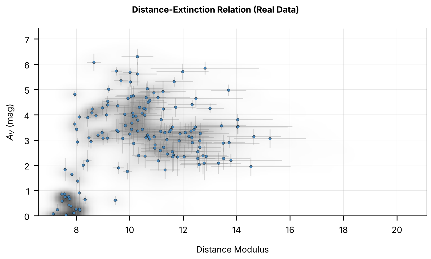
The LOS fitter works with posterior samples from BruteForce fits. Each star contributes distance and extinction samples that collectively trace the distance-reddening relation along the sightline.

Let’s load stellar posteriors and examine the distance-extinction structure.

Note: The LOS dust fitting in this tutorial uses the dynesty nested sampling package. Install it with pip install dynesty if you don’t have it already.

# Try to load real stellar posterior samples or generate synthetic ones
try:
    # Try to find results from Tutorial 5 (Orion field, no-dust-prior fit)
    datafile = find_brutus_data_file("Orion_l209.1_b-19.9_mist_nodust.h5")

    with h5py.File(datafile, 'r') as f:
        # Load distance and extinction samples
        dist_samples = f['samps_dist'][:] if 'samps_dist' in f else None
        av_samples = f['samps_red'][:] if 'samps_red' in f else None
        chi2 = f['obj_chi2min'][:] if 'obj_chi2min' in f else None
        nbands = f['obj_Nbands'][:] if 'obj_Nbands' in f else None

        if dist_samples is not None and av_samples is not None:
            print(f"Loaded {len(dist_samples)} stellar posterior samples from file")

            # Apply a loose chi2 cut to remove poor fits
            if chi2 is not None and nbands is not None:
                from scipy.stats import chi2 as chi2_dist
                # Goodness-of-fit p-value, not chi2/Nbands.
                dof = np.maximum(nbands - 3, 1)
                pvals = chi2_dist.sf(chi2, dof)
                good = pvals > 1e-6  # drop only the worst fits
                dist_samples = dist_samples[good]
                av_samples = av_samples[good]
                print(f"  After p-value > 1e-6 cut: {len(dist_samples)} stars kept")

            # Convert distances to distance modulus for LOS fitting
            dm_samples = 5 * np.log10(dist_samples * 1000) - 5  # kpc to distance modulus

            source = "Real Data"
        else:
            raise ValueError("No distance/extinction samples in file")

            

except (FileNotFoundError, ValueError, KeyError) as e:

    # Generate synthetic samples
    print("Generating synthetic stellar samples...")
    print(f"  (Real data not available: {e})\n")
    
    n_stars = 50
    n_samples = 100

    # Create synthetic distance modulus samples
    # Simulate stars at various distances with measurement uncertainties
    true_dm = np.random.uniform(7, 10, n_stars)  # True distance moduli
    dm_error = np.random.uniform(0.1, 0.3, n_stars)  # Uncertainties

    dm_samples = np.zeros((n_stars, n_samples))
    for i in range(n_stars):
        dm_samples[i] = np.random.normal(true_dm[i], dm_error[i], n_samples)

    # Create synthetic extinction samples (correlated with distance)
    # Simulate a dust cloud at distance modulus ~8.5
    cloud_dm = 8.5
    cloud_width = 0.3

    av_samples = np.zeros((n_stars, n_samples))
    for i in range(n_stars):
        # Background extinction
        av_bg = 0.3

        # Add cloud extinction for stars behind it
        for j in range(n_samples):
            if dm_samples[i, j] > cloud_dm:
                av_cloud = 1.5 * (1 - np.exp(-(dm_samples[i, j] - cloud_dm) / cloud_width))
                av_samples[i, j] = av_bg + av_cloud + np.random.normal(0, 0.1)
            else:
                av_samples[i, j] = av_bg * (dm_samples[i, j] / cloud_dm) + np.random.normal(0, 0.1)

    av_samples = np.maximum(0, av_samples)  # No negative extinction
    source = "Synthetic"

print(f"Using {source} stellar samples:")
print(f"  Stars: {len(dm_samples)}")
print(f"  Samples per star: {dm_samples.shape[1]}")
print(f"  Distance modulus range: [{dm_samples.min():.1f}, {dm_samples.max():.1f}]")
print(f"  A_V range: [{av_samples.min():.2f}, {av_samples.max():.2f}] mag")

Loaded 207 stellar posterior samples from Orion_l209.1_b-19.9_mist_nodust.h5
  After p-value > 1e-6 cut: 148 stars kept (500 samples/star)
  Distance modulus range: [7.1, 20.6]
  A_V range: [0.00, 7.14] mag

# Distance-extinction relation from stellar posteriors
from brutus.plotting import bin_pdfs_distred

# --- Bin posteriors into 2D distance-reddening PDFs ---
# bin_pdfs_distred expects (n_objects, n_samples) arrays for distance (in kpc)
# and reddening. We pass (dists, reds, dreds) as a 3-tuple.
dist_kpc = 10**((dm_samples + 5) / 5) / 1000  # DM -> kpc
rv_dummy = 3.32 * np.ones_like(av_samples)  # placeholder R(V)

# Determine plot span from data
dm_lo, dm_hi = float(np.nanmin(dm_samples)) - 0.5, float(np.nanmax(dm_samples)) + 0.5
av_lo, av_hi = 0.0, max(2.0, float(np.nanmax(av_samples)) + 0.3)
dist_lo = 10**((dm_lo + 5) / 5) / 1000
dist_hi = 10**((dm_hi + 5) / 5) / 1000

binned, xedges, yedges = bin_pdfs_distred(
    (dist_kpc, av_samples, rv_dummy),
    dist_type='distance_modulus',
    avlim=(av_lo, av_hi),
    span=((av_lo, av_hi), (dist_lo, dist_hi)),
    bins=(300, 150),
    smooth=0.02,
)
# binned shape: (n_stars, n_xbins, n_ybins) where x=DM, y=A_V

# Compute bin centers
xc = 0.5 * (xedges[:-1] + xedges[1:])  # distance modulus
yc = 0.5 * (yedges[:-1] + yedges[1:])  # A_V

# --- Build stacked 2D density (sum over all stars) ---
stacked = binned.sum(axis=0)

# --- Plot: single panel only (no marginals) ---
fig, ax_main = plt.subplots(figsize=(10, 6))

# Main panel: stacked 2D density + scatter
ax_main.pcolormesh(xedges, yedges, stacked.T, cmap='Greys', alpha=0.7)

# Overlay per-star medians
dm_median = np.median(dm_samples, axis=1)
dm_std = np.std(dm_samples, axis=1)
av_median = np.median(av_samples, axis=1)
av_std = np.std(av_samples, axis=1)
ax_main.errorbar(dm_median, av_median, xerr=dm_std, yerr=av_std,
                 fmt='none', ecolor='gray', alpha=0.3, zorder=1)
ax_main.scatter(dm_median, av_median, c='steelblue', s=20, zorder=5,
                edgecolor='k', linewidth=0.3)
ax_main.set_xlabel('Distance Modulus')
ax_main.set_ylabel('$A_V$ (mag)')
ax_main.set_ylim(bottom=0)
ax_main.grid(True, alpha=0.3)

fig.suptitle(f'Distance-Extinction Relation ({source})', fontsize=14, fontweight='bold')
plt.tight_layout()
save_figure(fig, 'stellar_samples')
plt.show()

Fitting a LOS Dust Model with Dynesty

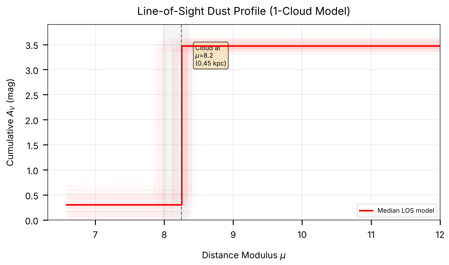
Nested sampling of the line-of-sight dust profile uses a prior transform and a sample-based log-likelihood:

• los_clouds_priortransform(u, rlims, dlims): Transforms unit cube draws into physical parameters. For an \(n\)-cloud model the parameter vector has \(2n + 4\) elements: \([p_b, s_{\text{fore}}, s_{\text{back}}, A_{V,\text{fore}}, d_1, A_{V,1}, \ldots, d_n, A_{V,n}]\).

• los_clouds_loglike_samples(theta, dsamps, rsamps, ...): Evaluates the log-likelihood of the cloud model given stellar distance and reddening posterior samples.

For a 1-cloud model (ndim=6), the parameters are:

Parameter	Meaning
\(p_b\)	Outlier fraction
\(s_{\text{fore}}\)	Foreground smoothing scale
\(s_{\text{back}}\)	Background smoothing scale
\(A_{V,\text{fore}}\)	Foreground extinction (before cloud)
\(d_1\)	Cloud distance (distance modulus)
\(A_{V,1}\)	Total extinction (after cloud)

We now run a nested sampling fit on the stellar posteriors.

# Run LOS dust fit with dynesty
from brutus.analysis import los_clouds_priortransform, los_clouds_loglike_samples
import dynesty
from dynesty.utils import resample_equal

# Set up 1-cloud model (ndim = 6)
ndim = 6

# Determine appropriate bounds from the data
dm_range = (float(dm_samples.min()) - 0.5, float(dm_samples.max()) + 0.5)
av_range = (0.0, max(3.0, float(av_samples.max()) + 0.5))

print(f"LOS fit setup:")
print(f"  Model: 1-cloud ({ndim} parameters)")
print(f"  Stars: {dm_samples.shape[0]}")
print(f"  Samples per star: {dm_samples.shape[1]}")
print(f"  Distance modulus bounds: [{dm_range[0]:.1f}, {dm_range[1]:.1f}]")
print(f"  A_V bounds: [{av_range[0]:.1f}, {av_range[1]:.1f}]")

def prior_transform(u):
    return los_clouds_priortransform(u, rlims=av_range, dlims=dm_range)

def loglike(theta):
    return los_clouds_loglike_samples(
        theta, dm_samples, av_samples,
        kernel='gauss', rlims=av_range, Ndraws=25, monotonic=True
    )

# Run nested sampling (rslice sampler is more efficient for this problem)
import time
t0 = time.time()
sampler = dynesty.NestedSampler(loglike, prior_transform, ndim,
                                nlive=200, sample='rslice')
sampler.run_nested(print_progress=False, maxcall=250000)
results = sampler.results
t_run = time.time() - t0

print(f"  Completed in {t_run:.1f}s")
print(f"  Log-evidence: {results.logz[-1]:.1f} +/- {results.logzerr[-1]:.1f}")
print(f"  Iterations: {results.niter}")

# Extract weighted posterior
weights = np.exp(results.logwt - results.logz[-1])
weights /= weights.sum()
posterior = resample_equal(results.samples, weights)

param_names = ['P_b', 's_fore', 's_back', 'A_V_fore', 'd_cloud (DM)', 'A_V_total']
print(f"\nPosterior summary (median [16th, 84th]):")
for i, name in enumerate(param_names):
    med = np.median(posterior[:, i])
    lo, hi = np.percentile(posterior[:, i], [16, 84])
    print(f"  {name:20s}: {med:.3f}  [{lo:.3f}, {hi:.3f}]")

# Convert cloud distance to kpc
dm_cloud = np.median(posterior[:, 4])
dist_kpc = 10**((dm_cloud + 5) / 5) / 1000
delta_av = np.median(posterior[:, 5] - posterior[:, 3])
print(f"\nCloud properties:")
print(f"  Distance: {dist_kpc:.2f} kpc (DM = {dm_cloud:.1f})")
print(f"  Foreground A_V: {np.median(posterior[:, 3]):.3f} mag")
print(f"  Extinction jump at cloud: {delta_av:.3f} mag")

LOS fit setup: 1-cloud model (6 parameters), 148 stars x 500 samples
  Completed in 41.2s (2564 iterations, log-evidence = -309.4 +/- 0.2)

Posterior summary (median [16th, 84th]):
  P_b                 : 0.088  [0.062, 0.121]
  s_fore              : 0.043  [0.025, 0.069]
  s_back              : 0.114  [0.101, 0.126]
  A_V_fore            : 0.307  [0.112, 0.510]
  d_cloud (DM)        : 8.250  [7.978, 8.361]
  A_V_total           : 3.476  [3.382, 3.580]

Cloud properties:
  Distance: 0.45 kpc (DM = 8.2)
  Foreground A_V: 0.307 mag
  Extinction jump at cloud: 3.163 mag

# Visualize the LOS dust fit results
fig, ax = plt.subplots(figsize=(10, 6))

# --- Foreground: LOS model step functions from dynesty posterior ---
# Each posterior sample defines: A(V) = Av_fore for d < d1,
#                                A(V) = Av_total for d >= d1
# Parameters: [p_b, s_fore, s_back, Av_fore, d1, Av_total]
dm_grid = np.linspace(xedges[0], 12, 500)

n_plot = min(200, len(posterior))
plot_idx = np.random.choice(len(posterior), n_plot, replace=False)

for k in plot_idx:
    av_fore_k = posterior[k, 3]
    d_cloud_k = posterior[k, 4]
    av_total_k = posterior[k, 5]
    step = np.where(dm_grid < d_cloud_k, av_fore_k, av_total_k)
    ax.step(dm_grid, step, where='post', color='red', alpha=0.03, lw=0.5)

# Median model step function
av_fore_med = np.median(posterior[:, 3])
d_cloud_med = np.median(posterior[:, 4])
av_total_med = np.median(posterior[:, 5])
step_med = np.where(dm_grid < d_cloud_med, av_fore_med, av_total_med)
ax.step(dm_grid, step_med, where='post', color='red', lw=2.5,
        label='Median LOS model', zorder=5)

# Mark cloud location
dm_cloud_lo, dm_cloud_hi = np.percentile(posterior[:, 4], [16, 84])
ax.axvline(d_cloud_med, color='k', ls='--', alpha=0.5, lw=1.5)
ax.axvspan(dm_cloud_lo, dm_cloud_hi, alpha=0.08, color='gray')

dist_kpc_med = 10**((d_cloud_med + 5) / 5) / 1000
ax.text(d_cloud_med + 0.2, ax.get_ylim()[1] * 0.9,
        f'Cloud at\n$\mu$={d_cloud_med:.1f}\n({dist_kpc_med:.2f} kpc)',
        fontsize=10, va='top',
        bbox=dict(boxstyle='round', facecolor='wheat', alpha=0.8))

ax.set_xlabel('Distance Modulus $\mu$')
ax.set_ylabel('Cumulative $A_V$ (mag)')
ax.set_title('Line-of-Sight Dust Profile (1-Cloud Model)')
ax.set_xlim(right=12)
ax.set_ylim(bottom=0)
ax.legend(loc='lower right', fontsize=10)
ax.grid(True, alpha=0.3)

plt.tight_layout()
save_figure(fig, 'los_dust_fit')
plt.show()

Summary and Key Takeaways

Key Concepts

1. LOS Dust Modeling (brutus.analysis.los_dust)

   • Multi-cloud models fit discrete dust structures along the line of sight.

   • The prior transform and log-likelihood interface directly with nested sampling (dynesty).

   • Evidence (\(\ln Z\)) values compare models with different cloud counts. When monotonic=True (the default), non-monotonic profiles are rejected inside the likelihood rather than the prior transform, shrinking the sampled prior volume; add back the mode-dependent volume offset (\(\ln[(n+1)!]\) for an \(n\)-cloud fit in the default mode) to each \(\ln Z\) before comparing models (see los_clouds_loglike_samples).

2. Stellar Posteriors

   • Per-star distance and extinction samples trace the cumulative distance-reddening relation.

   • bin_pdfs_distred bins and smooths individual stellar posteriors onto a shared 2-D grid.

Next Steps

• Tutorial 8: Photometric Calibration

• Fit 2-cloud and 3-cloud models and compare their corrected \(\ln Z\) values.

• Apply LOS fitting across multiple sightlines to build a 3D dust map.