Tutorials / Classifier outputs: class fractions under label shift

Classifier outputs: class fractions under label shift

A classifier is trained on one set of objects and applied to another, whose class fractions differ. This change is label shift. The fractions of the classes in the new set, \(\rho_k\) (the prevalence), are what binference infers. This tutorial follows two routes, named by what you have:

• posteriors and the training prevalence: the classifier’s class probabilities and the class fractions it was trained with;

• scores and a labelled set: any score from the classifier, and a labelled set that shows how each class scores.

import matplotlib.pyplot as plt
import numpy as np

import binference
from binference.plotting import SAMPLE_COLOR

Posteriors and the training prevalence

A classifier trained on balanced classes is applied to a set whose classes are skewed. Its probability \(P_{ik}\) that object \(i\) is in class \(k\) includes the training prevalence \(\Pi_k\) as a prior. binference.simulate.mock_categorical() simulates a calibrated classifier on four overlapping classes:

mock = binference.simulate.mock_categorical(3000, n_classes=4, separation=1.2, rng=5)
probs, train_prior = mock.posteriors, mock.interim
print("true class fractions:", mock.truth.rho.round(3), " training prevalence:", train_prior)

true class fractions: [0.033 0.133 0.3   0.533]  training prevalence: [0.25 0.25 0.25 0.25]

Two shortcuts are common. “Classify and count” assigns each object to its most probable class and counts. “Probabilistic classify and count” averages the probabilities. Both are biased toward the training prevalence. binference treats the training prevalence as the interim prior and divides it out. This is the Bayesian form of the EM method of Saerens et al. (2002):

lk = binference.Likelihoods.from_table(probs, mock.bins, interim=train_prior)
fit = binference.infer(lk, rng=1)

cc = np.bincount(probs.argmax(axis=1), minlength=4) / len(probs)
pcc = probs.mean(axis=0)
lo, hi = fit.interval(0.95)
for k, name in enumerate(mock.bins.labels):
    print(f"{name}: truth {mock.truth.rho[k]:.3f} | CC {cc[k]:.3f} | PCC {pcc[k]:.3f} | "
          f"binference {fit.mean[k]:.3f} [{lo[k]:.3f}, {hi[k]:.3f}]")

class_0: truth 0.033 | CC 0.076 | PCC 0.094 | binference 0.036 [0.020, 0.053]
class_1: truth 0.133 | CC 0.155 | PCC 0.178 | binference 0.140 [0.098, 0.185]
class_2: truth 0.300 | CC 0.294 | PCC 0.302 | binference 0.271 [0.209, 0.330]
class_3: truth 0.533 | CC 0.476 | PCC 0.426 | binference 0.553 [0.515, 0.591]

fig, ax = plt.subplots()
fit.plot(ax=ax, which="fractions", truth=mock.truth.rho, stack=pcc, sample_color=SAMPLE_COLOR,
         label="binference")
ax.legend(ncol=2, loc="lower left", bbox_to_anchor=(0, 1))
ax.set_xlabel("class");

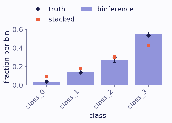
Class fractions inferred by binference (bars with 68% intervals), the truth (diamonds) and the averaged probabilities (squares).

The averaged probabilities, labelled “stacked”, lie closer to equal fractions than the truth does.

Each object’s posterior under the inferred fractions, fit.assignment_probabilities(), is the classifier’s output recalibrated to the new set. Use it to classify objects in the new set:

recal = fit.assignment_probabilities()
acc_before = np.mean(probs.argmax(axis=1) == mock.truth.labels)
acc_after = np.mean(recal.argmax(axis=1) == mock.truth.labels)
print(f"accuracy with the classifier's probabilities: {acc_before:.3f}, recalibrated: {acc_after:.3f}")

accuracy with the classifier's probabilities: 0.607, recalibrated: 0.654

Scores and a labelled set

Dividing out the training prevalence is exact only when the probabilities are calibrated. A labelled set gives a route that needs no calibration (inputs guide). Bin the classifier’s score, and tally how each class of the labelled set falls into the score bins with from_labelled(). The tally is a response matrix \(R_{jk}\): the probability of score bin \(j\) for an object of class \(k\). The new set then enters as a binned measurement.

Here the mock halves the classifier’s log-likelihoods (temperature=2), so its probabilities are too flat. The score is the object’s one-dimensional feature:

flat = binference.simulate.mock_categorical(
    3000, n_classes=4, separation=1.2, temperature=2.0, n_validation=2000, rng=5
)
lk_post = binference.Likelihoods.from_table(flat.posteriors, flat.bins, interim=flat.interim)
lk_score = binference.Likelihoods.from_binned(flat.response, values=flat.measurements["feature"])
fit_post = binference.infer(lk_post, rng=1)
fit_score = binference.infer(lk_score, rng=1)
print(flat.response)
print("truth                      ", flat.truth.rho.round(3))
print("posteriors and prevalence  ", fit_post.mean.round(3))
print("scores and a labelled set  ", fit_score.mean.round(3))

Response(J=10 measured bins, K=4 truth bins, from labelled data)
truth                       [0.033 0.133 0.3   0.533]
posteriors and prevalence   [0.007 0.008 0.621 0.364]
scores and a labelled set   [0.035 0.142 0.28  0.543]

The mock built flat.response with Response.from_labelled(scores, labels) from its labelled set of 2000 objects. The scores route lands closer to the truth than the posteriors route, whose flat probabilities bias it. infer also tests whether label shift holds; the inputs guide describes the test.

What to take away

• With calibrated probabilities, pass them with the training prevalence: Likelihoods.from_table(probs, Bins.categories(classes), interim=train_prior).

• With a labelled set, tally the scores with Response.from_labelled and pass the new set’s scores to Likelihoods.from_binned. This route does not need calibration.

• Mixed-stock analysis uses the labelled-set route with a confusion matrix. The quantification background page places both routes in that field.