Tutorials / Posterior samples: black-hole masses

Posterior samples: black-hole masses

Gravitational-wave catalogues describe each detected merger by posterior samples of its parameters. The samples come from a parameter-estimation (PE) run, which used a prior of its own: the PE prior. This tutorial infers the distribution of black-hole masses from such samples. It shows why the PE prior must be divided out, and how many samples each event needs.

import warnings

import matplotlib.pyplot as plt
import numpy as np
from scipy import stats

import binference

A simulated catalogue

The primary masses \(m\) of the mergers follow a power law \(p(m)\propto m^{-2.3}\) between 5 and 85 solar masses (90% of mergers), plus a Gaussian peak at 34 solar masses with width 4 (10%). Each of 600 events has a measured \(\ln m\) with a Gaussian error between 0.2 and 0.4.

The PE runs used a prior uniform in the two component masses. For the heavier one this makes the prior roughly proportional to \(m\), so it favours heavy masses. In \(\ln m\) the prior density is proportional to \(m^2\).

binference.simulate.mock_1d() works in \(\ln m\). It draws 1000 samples per event from the event’s posterior under the PE prior. A catalogue would publish them in solar masses, so the code converts them:

m_lo, m_hi, slope = 5.0, 85.0, -2.3

def population(x):                       # density of ln m
    m, a = np.exp(x), slope + 1
    power_law = a * m**slope / (m_hi**a - m_lo**a)
    return (0.9 * power_law + 0.1 * stats.norm.pdf(m, 34.0, 4.0)) * m

ln_bins = binference.Bins.linear(np.log(m_lo), np.log(m_hi), 16)
mock = binference.simulate.mock_1d(
    600, ln_bins, density=population, noise=(0.2, 0.4),
    interim=lambda x: np.exp(2 * x),     # the PE prior: proportional to m**2 in ln m
    n_samples=1000, rng=150914,
)
samples = np.exp(mock.samples)           # (events, samples), in solar masses
rho_true = mock.truth.rho
print(samples.shape, "median mass of the first events:", np.median(samples[:4], axis=1).round(1))

(600, 1000) median mass of the first events: [43.8  7.4  9.1 11.1]

The bins are 16 intervals of equal width in \(\ln m\). Bins.log makes them in \(m\) itself, so the samples go in as they are:

bins = binference.Bins.log(m_lo, m_hi, 16)
print(bins)

Bins(K=16, range=(5, 85), measure=log)

Dividing out the PE prior

from_samples() turns each event’s samples into bin-averaged likelihoods. It weights each sample by the inverse of the PE prior, which is passed as a function of \(m\). The tempting shortcut passes interim="flat", as if the samples came from the likelihood:

lk = binference.Likelihoods.from_samples(samples, bins, interim=lambda m: m)
lk_flat = binference.Likelihoods.from_samples(samples, bins, interim="flat")

kw = dict(rng=1, n_samples=500, n_warmup=300)   # shorter runs than the default, for speed
fits = {"PE prior divided out": binference.infer(lk, **kw),
        "PE prior ignored": binference.infer(lk_flat, **kw)}

fig, axes = plt.subplots(2, 1, sharex=True, sharey=True)
fig.set_figheight(5.1)
for ax, (name, fit), color in zip(axes, fits.items(), ["C0", "C1"]):
    fit.plot(ax=ax, which="fractions", truth=rho_true, color=color, label="median")
    ax.set_title(name, loc="left")
    ax.set_xscale("log")
axes[0].set_xlabel("")
axes[0].legend(loc="upper right")
axes[1].get_legend().remove()
axes[1].set_xticks([5, 10, 20, 40, 80], ["5", "10", "20", "40", "80"], minor=False)
axes[1].minorticks_off()
axes[1].set_xlabel(r"primary mass $m$ [$M_\odot$]");

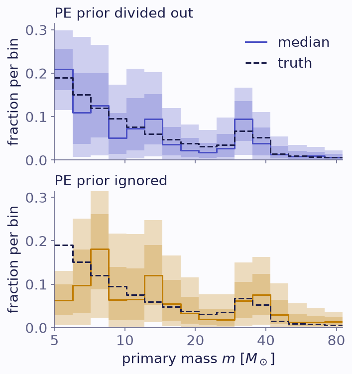
Population fractions of the primary mass, with 68% and 95% bands. The PE prior is divided out (top) or ignored (bottom). The truth is dashed; the mass axis is logarithmic.

Ignoring the PE prior moves the population toward heavy masses, where that prior is large. The mean of \(\ln m\) over the population shows the size of the shift, in units of its posterior standard deviation:

ln_m = np.log(bins.centers)              # ln m at the bin centres
mean_ln_m = {name: fit.functional(lambda rho: rho @ ln_m) for name, fit in fits.items()}
for name, g in mean_ln_m.items():
    print(f"{name:21s} {g.mean():.3f} ± {g.std():.3f}")
print(f"{'truth':21s} {rho_true @ ln_m:.3f}")
g_right, g_flat = mean_ln_m.values()
print(f"shift from ignoring the PE prior: {(g_flat.mean() - g_right.mean()) / g_flat.std():.1f} sd")

PE prior divided out  2.460 ± 0.031
PE prior ignored      2.630 ± 0.031
truth                 2.430
shift from ignoring the PE prior: 5.5 sd

Each sample carries the PE prior. The interim prior of the inputs guide is the same thing under a general name. A catalogue states it with the samples; check it before you fit.

How many samples each event needs

A likelihood built from samples is a Monte Carlo estimate, so it carries noise. With 1000 samples per event the noise is small: the fit agrees with one from the exact likelihoods, which a real analysis does not have.

exact = binference.infer(mock.likelihoods, **kw)
shift = np.abs(fits["PE prior divided out"].mean - exact.mean) / exact.std
print(f"largest shift from the exact fit: {shift.max():.2f} posterior sd")

largest shift from the exact fit: 0.40 posterior sd

With 30 samples per event the estimates are noisy. binference warns about the inputs twice: when it builds the likelihoods, and when it checks the fit. The second warning measures the Monte Carlo variance \(V_i(\rho)\) of each event’s likelihood at the fitted population. It fires when their sum exceeds the threshold on the defaults page:

with warnings.catch_warnings(record=True) as caught:
    warnings.simplefilter("always")
    lk_30 = binference.Likelihoods.from_samples(samples[:, :30], bins, interim=lambda m: m)
    fit_30 = binference.infer(lk_30, **kw)
for w in caught:
    if issubclass(w.category, binference.InputWarning):
        print(w.message, end="\n\n")

for name, l, fit in [("1000 samples", lk, fits["PE prior divided out"]),
                     ("30 samples", lk_30, fit_30)]:
    V, _ = l.sample_variance(fit.mean)
    print(f"{name}: sum of V_i = {V.sum():.1f}")

81 of 600 objects have fewer than 20 effective samples inside the bins; their likelihoods will be noisy (more samples, wider bins or floor= help).

Diagnostics: likelihoods from samples carry Monte Carlo variance sum_i V_i = 19 > 1 at the fitted population. Hint: draw more samples per object, or use wider bins or floor=.

1000 samples: sum of V_i = 0.7
30 samples: sum of V_i = 18.7

If the sum is large, use more samples per event or wider bins; the inputs guide lists the other options.

What to take away

• Pass the PE prior to from_samples(). Give it in the coordinate of the samples; with log bins, binference handles the change to \(\ln m\).

• Check the Monte Carlo variance of the likelihoods, \(\sum_iV_i\), before you trust the fit. binference warns when it is too large.

• This catalogue was complete. Real detectors miss light mergers more often than heavy ones; Selection measured by injections corrects for that. The gravitational-wave background page maps the field’s formulas onto binference.