Tutorials / Binned counts and a response: unfolding a spectrum

Binned counts and a response: unfolding a spectrum

A detector records each event in a measured bin \(j\), such as a bin of reconstructed energy. An event with a true value in bin \(k\) lands in measured bin \(j\) with probability \(R_{jk}\), the response matrix. Some events are lost entirely, so the efficiency \(\epsilon_k=\sum_jR_{jk}\) is less than one. Recovering the true spectrum from the counts is unfolding. This tutorial unfolds a smeared spectrum with binference, under a Dirichlet prior and under a smoothness prior.

import matplotlib.pyplot as plt
import numpy as np
from matplotlib.colors import LinearSegmentedColormap, to_rgb

import binference
from binference.plotting import SAMPLE_COLOR

The response and the counts

binference.simulate.mock_unfolding() smears an exponential spectrum of 8000 events. It has 20 true bins and 25 measured bins:

mu = binference.simulate.mock_unfolding(8000, n_true=20, n_reco=25, rng=3)
R = mu.response.matrix                   # (measured bins, true bins)
counts = mu.measurements["reco_counts"]

fig, axes = plt.subplots(2, 1, height_ratios=[1.4, 1])
fig.set_figheight(5.8)
c0, ground = np.array(to_rgb("C0")), np.array(to_rgb(plt.rcParams["axes.facecolor"]))
ramp = LinearSegmentedColormap.from_list("ramp", [0.15 * c0 + 0.85 * ground, c0])
im = axes[0].imshow(R, origin="lower", aspect="auto", cmap=ramp)
axes[0].set(xlabel="true bin k", ylabel="measured bin j")
fig.colorbar(im, ax=axes[0], label="$R_{jk}$")
axes[1].stairs(counts, np.arange(len(counts) + 1) - 0.5, color=SAMPLE_COLOR, lw=1.8)
axes[1].set(xlabel="measured bin j", ylabel="events");

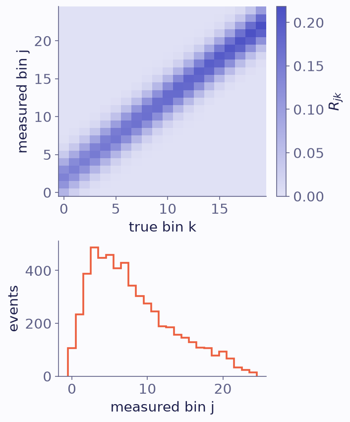
The response matrix (top), and the counts of detected events in the measured bins (bottom).

from_binned() turns the counts and the response into likelihood rows, one per measured bin, weighted by the counts. Each event measured in bin \(j\) gets the row \(R_{j\cdot}\). The efficiency enters as a selection on the measurement, because the response already includes it.

Inverting \(R\) directly amplifies the noise. Least squares on these counts gives “fractions” that swing between large positive and negative values:

naive, *_ = np.linalg.lstsq(R, counts, rcond=None)    # unregularised inversion
naive = naive / naive.sum()
print("matrix inversion, normalised:", naive[:6].round(1), "...")

matrix inversion, normalised: [  0.2  -0.4   2.8  -6.9  13.5 -21.6] ...

A smoothness prior regularises the unfolding: it stops the noise from growing. It infers how smooth the spectrum is, instead of fixing an iteration count or a regularisation strength by hand. Both fits use NUTS, with the chains in parallel processes:

lk = binference.Likelihoods.from_binned(mu.response, counts=counts)
print(lk, lk.selection)
flat = binference.infer(lk, method="nuts", rng=1, n_chains=2, n_warmup=400, n_samples=500,
                        n_jobs=-1)
smooth = binference.infer(lk, binference.priors.LogisticGP(), method="nuts", rng=1,
                          n_warmup=500, n_samples=500, n_jobs=-1, check=False)
d = smooth.diagnostics
print(f"divergent: {d['n_divergent']} of {smooth.n_draws}, max R-hat {d['rhat'].max():.3f}, "
      f"min bulk ESS {d['ess_bulk'].min():.0f}")

Likelihoods(N=25, K=20, dense, W=5456, selection='on_measurement', bins=Bins(K=20, range=(0, 1))) Selection(K=20, mode='on_measurement', scale='probability')
divergent: 0 of 2000, max R-hat 1.004, min bulk ESS 1560

check=False stops infer from warning, so that the diagnostics can be read here. The largest R-hat is below 1.01 and the smallest bulk effective sample size is above 400. Divergent transitions, if any, are rare; the pitfalls guide says when they matter.

The unfolded spectrum

truth = mu.truth.rho
fig, axes = plt.subplots(2, 1, sharex=True, sharey=True)
fig.set_figheight(5.1)
flat.plot(ax=axes[0], truth=truth, which="fractions", label="median")
smooth.plot(ax=axes[1], truth=truth, which="fractions", label="median")
axes[0].set_title("Dirichlet prior", loc="left")
axes[1].set_title("Gaussian-process prior", loc="left")
axes[0].legend(loc="upper right")
axes[1].get_legend().remove()
axes[0].set_xlabel("")
axes[1].set_xlabel("true value");

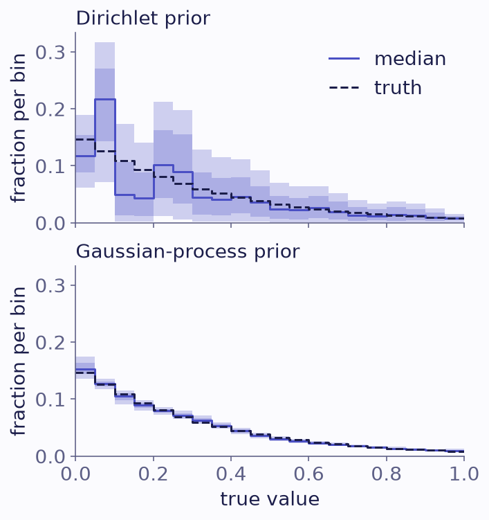
The unfolded spectrum as population fractions, with 68% and 95% bands, under a Dirichlet prior (top) and a Gaussian-process prior (bottom). The truth is dashed.

The bands show the uncertainty that unfolding methods often leave out. The smoothness prior learns its own amplitude and length scale from the data:

for name, draws in smooth.info["hyperparameters"].items():
    print(f"{name}: {np.quantile(draws, [0.16, 0.5, 0.84]).round(2)}")

amplitude: [0.9  1.3  1.93]
length_scale: [0.4  0.57 0.85]

Tip

An order-2 random walk (LogisticRandomWalk(order=2)) is another natural prior here. But this spectrum is an exact exponential, and its log is a straight line, which the order-2 random walk does not penalise at all. The posterior then pushes the walk’s scale toward zero. This narrow region of the posterior makes NUTS report divergences. A Gaussian-process prior, target_accept=0.95, or a scale hyperprior bounded away from zero avoids it.

What to take away

• Counts in measured bins and a response enter through Likelihoods.from_binned(response, counts=counts), which also attaches the efficiency.

• A smoothness prior regularises the unfolding and infers its own strength.

• The inputs guide shows how to build a response from simulated events. The unfolding background page relates this to the methods of particle physics.