Tutorials / Validating an analysis

Validating an analysis

Convergence diagnostics say whether a sampler explored the posterior. They do not say whether the posterior is calibrated. This tutorial checks a whole pipeline with binference’s validation tools: an exact reference for a small problem, simulation-based calibration (SBC), and coverage. It also shows what a failure looks like.

import warnings

import numpy as np

import binference
from binference import priors
from binference.validation import coverage, exact_posterior, sbc

Exact posteriors

With three bins, binference can integrate the posterior on a grid. Here it compares that exact posterior with NUTS and Gibbs, on data with a selection:

bins = binference.Bins([0.0, 1.0, 2.0, 3.0])
S = np.array([0.9, 0.5, 0.25])
mock = binference.simulate.mock_1d(250, bins, density=np.array([0.4, 0.35, 0.25]),
                               noise=(0.3, 0.8), selection=S, rng=777)
exact = exact_posterior(mock.likelihoods, priors.Dirichlet(1.0))
nuts = binference.infer(mock.likelihoods, method="nuts", rng=1)
gibbs = binference.infer(mock.likelihoods, method="gibbs", rng=1, n_samples=4000)
print("exact mean", exact.mean.round(4), " sd", exact.std.round(4))
print("NUTS  mean", nuts.mean.round(4), " sd", nuts.std.round(4))
print("Gibbs mean", gibbs.mean.round(4), " sd", gibbs.std.round(4))

exact mean [0.4071 0.3173 0.2756]  sd [0.0429 0.0642 0.0601]
NUTS  mean [0.4072 0.3164 0.2765]  sd [0.0416 0.0632 0.0588]
Gibbs mean [0.4077 0.3209 0.2714]  sd [0.0424 0.0651 0.062 ]

The theory page describes the test suite’s comparisons.

Simulation-based calibration

SBC (Talts et al. 2018) checks the whole loop of prior, simulator and inference (simulation-based calibration). Here it checks 150 fits of 50 objects in four bins. The measurement errors are 0.1, less than half a bin, so that every Gibbs fit converges in a short run:

prior = priors.Dirichlet(1.0)
grid = binference.Bins.linear(0.0, 1.0, 4)
simulate = binference.simulate.prior_predictive(prior, grid, n_objects=50, noise=0.1)

def fit_gibbs(lk, rng):
    return binference.infer(lk, prior, method="gibbs", rng=rng, n_chains=4,
                        n_warmup=200, n_samples=500, check=False)

result = sbc(simulate, fit_gibbs, n_simulations=150, n_draws=19, rng=0)
print("uniformity p-values:",
      {n: round(float(v), 3) for n, v in zip(result.names, result.pvalues(10))})

uniformity p-values: {'rho[0]': 0.893, 'rho[1]': 0.936, 'rho[2]': 0.057, 'rho[3]': 0.534, 'loglike': 0.35}

result.plot();

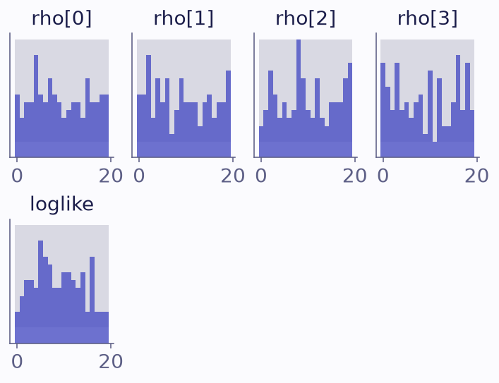
SBC rank histograms of the four fractions and of the log-likelihood of the true population (last panel), for Gibbs. The grey band holds 99% of histograms of uniform ranks.

The rank histograms sit inside the band expected for uniform ranks. The last panel ranks the log-likelihood of the true population. It is sensitive to errors in the correlations between bins, which per-bin ranks can miss.

What a failure looks like

Mean-field VB is over-confident, so the true value falls outside the bulk of its draws too often. It is most over-confident when the likelihoods are broad, so this check uses errors of 0.25, as wide as a bin. The rank histograms of the fractions become U-shaped:

def fit_vb(lk, rng):
    with warnings.catch_warnings():
        warnings.simplefilter("ignore", binference.ApproximationWarning)
        return binference.infer(lk, prior, method="vb", rng=rng, n_samples=1000)

simulate_broad = binference.simulate.prior_predictive(prior, grid, n_objects=50, noise=0.25)
bad = sbc(simulate_broad, fit_vb, n_simulations=150, n_draws=19, rng=0)
print("uniformity p-values:",
      {n: round(float(v), 4) for n, v in zip(bad.names, bad.pvalues(10))})

uniformity p-values: {'rho[0]': 0.0, 'rho[1]': 0.0, 'rho[2]': 0.0, 'rho[3]': 0.0, 'loglike': 0.0}

bad.plot();

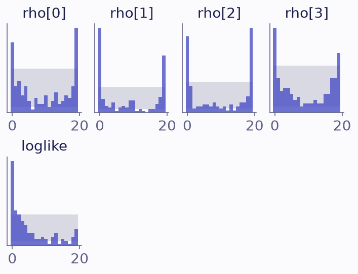
SBC rank histograms for mean-field VB. The grey band holds 99% of histograms of uniform ranks.

Coverage

Coverage asks how often central credible intervals contain the truth. With data simulated from the prior, Bayesian intervals have their nominal coverage on average. coverage checks any derived quantity, here the population mean:

centers = grid.centers
cov = coverage(simulate, fit_gibbs, n_simulations=150, levels=(0.5, 0.9),
               functionals={"mean": lambda rho: rho @ centers}, rng=1)
rates = cov.coverage_rates()                   # (levels, quantities)
se = cov.stderr().ravel()                      # one standard error per level
print(f"{'level':>6s}" + "".join(f"{n:>8s}" for n in cov.names))
for level, row, e in zip(cov.levels, rates, se):
    print(f"{level:6.2f}" + "".join(f"{r:8.2f}" for r in row) + f"   (standard error {e:.3f})")
z = (rates - np.array(cov.levels)[:, None]) / se[:, None]
print(f"deviation from nominal, in standard errors: mean {z.mean():.1f}, largest {np.abs(z).max():.1f}")

 level  rho[0]  rho[1]  rho[2]  rho[3]    mean
  0.50    0.50    0.45    0.48    0.49    0.44   (standard error 0.041)
  0.90    0.90    0.85    0.89    0.92    0.88   (standard error 0.024)
deviation from nominal, in standard errors: mean -0.6, largest 1.9

Each rate lies within about two standard errors of its level, as it should for a calibrated fit.

Validating your own pipeline

To check your own analysis, simulate catalogues like yours and call sbc or coverage with the settings of the real fit (mock catalogues).