Tutorials / Empirical Bayes deconvolution

Empirical Bayes deconvolution

Many problems in statistics share one shape. There are many units \(i=1,\dots,N\), each with an unknown effect \(z_i\). Each has a noisy estimate \(d_i\sim\mathcal N(z_i, \sigma_i^2)\) with a known standard error \(\sigma_i\). The units might be genes, schools, hospitals or baseball players. Estimating the distribution of the effects from the \(d_i\) is deconvolution. Using that distribution as a prior for each unit is empirical Bayes. Its posterior means shrink each \(d_i\) toward where the other units lie.

On a grid of bins this is binference’s model. The distribution of the effects is the population \(\rho\) over bins of \(z\); the empirical Bayes literature calls it \(g\). Each unit’s likelihood is its Gaussian measurement. The nonparametric maximum-likelihood estimate (NPMLE) of Kiefer and Wolfowitz (1956) maximises the likelihood over all distributions of \(z\). This tutorial computes the NPMLE, the full posterior of \(\rho\), and the shrinkage estimates of the units that follow from each.

import matplotlib.pyplot as plt
import numpy as np
from matplotlib.colors import LinearSegmentedColormap, to_rgb
from scipy import stats

import binference
from binference.plotting import SAMPLE_COLOR

rng = np.random.default_rng(81)

Simulated effects

There are 1500 units. 60% of them have no effect, \(z_i=0\); the others have effects drawn from \(\mathcal N(2.5, 0.7^2)\). The standard errors are uniform between 0.5 and 1.5. That is comparable to the gap between the two groups, so the estimates of null and non-null units overlap.

n = 1500
null = rng.random(n) < 0.6
z = np.where(null, 0.0, rng.normal(2.5, 0.7, n))       # true effects
sigma = rng.uniform(0.5, 1.5, n)                        # standard errors
d = z + sigma * rng.standard_normal(n)                  # estimates
print(f"{null.sum()} null units; estimates range from {d.min():.2f} to {d.max():.2f}")

923 null units; estimates range from -5.44 to 7.74

The grid has 70 bins of width 0.1 on \([-2.05, 4.95]\), with one bin centred on zero. The true \(\rho\) in these bins is the point mass at zero plus the Gaussian’s mass in each bin:

bins = binference.Bins.linear(-2.05, 4.95, 70)
edges = bins.edges[0]
rho_true = 0.4 * np.diff(stats.norm.cdf(edges, 2.5, 0.7))
rho_true[bins.index(0.0)] += 0.6
rho_true /= rho_true.sum()             # the Gaussian's tails beyond the grid are dropped
lk = binference.Likelihoods.from_gaussian(d, sigma, bins)

The NPMLE and the posterior of the population

With the default flat Dirichlet prior, the MAP estimate is the maximum-likelihood estimate of \(\rho\) on the grid: the NPMLE restricted to the grid. method="map" computes it with mix-SQP, and reports the KKT gap, which is near zero at the maximum:

npmle = binference.infer(lk, method="map")
atoms = npmle.rho > 1e-3
print(f"KKT gap {npmle.kkt_gap:.1e}; {atoms.sum()} bins hold more than 0.1% of the mass")
for c, w in zip(bins.centers[atoms], npmle.rho[atoms]):
    print(f"  z = {c:5.2f}: {w:.3f}")

KKT gap 4.7e-11; 6 bins hold more than 0.1% of the mass
  z = -1.30: 0.006
  z =  0.00: 0.602
  z =  1.90: 0.235
  z =  3.20: 0.062
  z =  3.30: 0.092
  z =  4.90: 0.002

The NPMLE puts all its mass on a few grid points; theory says it always does. It finds the mass at zero but represents the Gaussian by a few spikes. It gives no measure of its own uncertainty. The default method="auto" samples the full posterior of \(\rho\):

fit = binference.infer(lk, n_samples=500, rng=1)
print(fit.info["auto_method"], "-", fit.info["auto_reason"])

nuts - the Laplace importance check failed

fig, ax = plt.subplots()
fit.plot(ax=ax, which="fractions", truth=rho_true, label="median")
ax.vlines(bins.centers[atoms], 0, npmle.rho[atoms], color="C1", lw=2.5, label="NPMLE")
ax.set(xlabel="effect $z$", ylim=(0, 0.35))
ax.legend(ncol=3, loc="lower left", bbox_to_anchor=(0, 1));

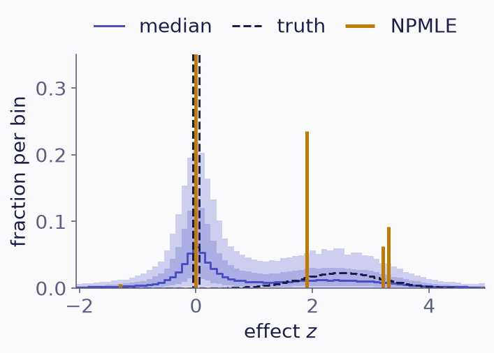
The posterior of the population fractions (median, 68% and 95% bands), the NPMLE’s atoms (vertical lines) and the truth (dashed). The truth’s spike at zero, 0.6, runs off the top.

The posterior bands are wide. The standard errors are 5 to 15 bins wide, so the data cannot tell a point mass at zero from a narrow bump around it. The posterior spreads the null mass over neighbouring bins. Sums over wider ranges are better determined than single bins:

near, mass = {}, {}
for cut in (0.5, 1.25):
    near[cut] = b = np.abs(bins.centers) < cut
    mass[cut] = m = fit.functional(lambda rho: rho[b].sum())
    print(f"mass within {cut} of zero: posterior {m.mean():.3f} ± {m.std():.3f}, "
          f"NPMLE {npmle.rho[b].sum():.3f}, truth {rho_true[b].sum():.3f}")
ratio = fit.prior_information_ratio()
print(f"prior information ratio: {ratio:.2f}")

mass within 0.5 of zero: posterior 0.445 ± 0.036, NPMLE 0.602, truth 0.601
mass within 1.25 of zero: posterior 0.614 ± 0.022, NPMLE 0.602, truth 0.615
prior information ratio: 1.98

Within 1.25 of zero, the posterior agrees with the truth. Within 0.5 it falls well short, while the NPMLE does not. The likelihood changes little when mass moves from the spike into the empty bins beside it. The posterior spreads along that direction, so its mean puts less mass on the spike. The prior information ratio (prior_information_ratio()) is above one. It says that the flat Dirichlet on 70 bins weighs more than the data in this fine structure. Ask about the null fraction as a sum over a range the data can resolve, or use a prior that expects a spike.

Shrinkage estimates for each unit

Each unit’s posterior under the estimated population is assignment_probabilities(): its probability of lying in each bin. For the NPMLE this is the usual plug-in empirical Bayes posterior. For the full fit it is averaged over the posterior draws of \(\rho\), so the uncertainty of the population carries into each unit. sample_values() draws the units’ true values, and their average is each unit’s posterior mean.

eb_npmle = npmle.assignment_probabilities() @ bins.centers   # bin centres, for the NPMLE
draws = fit.sample_values(rng=2)                  # (500 draws, units)
eb_full = draws.mean(axis=0)

For comparison, the oracle Bayes rule is the best possible estimate, which uses the true distribution of the effects. It integrates over \(z\) numerically:

grid = np.linspace(-6, 9, 3001)
dz = grid[1] - grid[0]
slab = 0.4 * stats.norm.pdf(grid, 2.5, 0.7)
like = stats.norm.pdf(d[:, None], grid, sigma[:, None])
oracle = (like @ (slab * grid)) * dz / ((like @ slab) * dz + 0.6 * stats.norm.pdf(d, 0, sigma))

mse = {name: np.mean((est - z) ** 2) for name, est in
       [("raw estimate d", d), ("EB, NPMLE", eb_npmle),
        ("EB, full posterior", eb_full), ("oracle Bayes", oracle)]}
for name, v in mse.items():
    print(f"{name:19s} mean squared error {v:.3f}")

raw estimate d      mean squared error 1.168
EB, NPMLE           mean squared error 0.527
EB, full posterior  mean squared error 0.552
oracle Bayes        mean squared error 0.522

Both empirical Bayes estimates more than halve the error of the raw estimates. They come close to the oracle that knows the true distribution. The plot shows the shrinkage. Estimates near zero move to zero, and those near the non-null group toward 2.5. Noisier units, the darker points, move further.

coral = np.array(to_rgb(SAMPLE_COLOR))   # from a pale tint to a dark shade of coral
ramp = LinearSegmentedColormap.from_list("ramp", [0.35 * coral + 0.65, coral, 0.5 * coral])
fig, ax = plt.subplots()
sc = ax.scatter(d, eb_full, c=sigma, s=8, cmap=ramp, lw=0)
ax.plot([-3, 7], [-3, 7], color="0.45", lw=1, ls="--")
ax.set(xlabel="raw estimate $d_i$", ylabel="posterior mean of $z_i$", xlim=(-3, 7),
       ylim=(-1, 5))
fig.colorbar(sc, ax=ax, label=r"standard error $\sigma_i$");

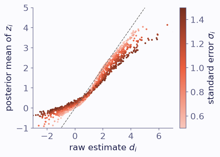
Each unit’s posterior mean against its raw estimate, shaded by its standard error. The dashed line marks no shrinkage.

The draws also give each unit an interval. Their coverage of the true effects checks the whole fit:

lo, hi = np.quantile(draws, [0.05, 0.95], axis=0)
covered = (z >= lo) & (z <= hi)
print(f"90% intervals cover {covered.mean():.3f} of the true effects; "
      f"mean width {np.mean(hi - lo):.2f}, against {2 * 1.645 * sigma.mean():.2f} for d ± 1.645 σ")
for name, units in [("null units", null), ("non-null units", ~null)]:
    se = np.sqrt(0.9 * 0.1 / units.sum())
    print(f"  {name:15s} cover {covered[units].mean():.3f} (standard error {se:.3f})")

90% intervals cover 0.941 of the true effects; mean width 2.37, against 3.27 for d ± 1.645 σ
  null units      cover 0.977 (standard error 0.010)
  non-null units  cover 0.882 (standard error 0.012)

The intervals cover more than 90% overall, and the null units explain it. The posterior spreads the spike at zero over the neighbouring bins, so a null unit’s interval is wide around zero and almost always contains it. The non-null units are covered at the nominal rate, within the standard error.

What to take away

• Deconvolution with known standard errors is binference’s model, with Likelihoods.from_gaussian on a grid of bins.

• method="map" with the default flat Dirichlet prior is the grid NPMLE. The full posterior of \(\rho\) shows how much of it the data determine.

• assignment_probabilities() and sample_values() give each unit’s empirical Bayes posterior, with the population’s uncertainty included.

• A smooth \(\rho\), as in Efron’s g-modelling, corresponds to a smoothness prior such as priors.LogisticGP() (Priors and smoothness). The empirical Bayes background page places this tutorial among the packages of that field.