Tutorials / Priors and smoothness

Priors and smoothness

When the data are sparse, the prior shapes the answer. Sparse means few objects per bin, or errors as wide as the bins. This tutorial puts four of binference’s priors side by side on a small catalogue. It shows how binference infers the smoothness hyperparameters, and uses held-out objects to choose between priors.

import warnings

import matplotlib.pyplot as plt
import numpy as np

import binference
from binference import priors

bins = binference.Bins.linear(0, 3, 40)
mock = binference.simulate.mock_1d(400, bins, noise=(0.05, 0.15), rng=21)
lk = mock.likelihoods
print(f"{lk.N} objects in {lk.K} bins: {lk.N / lk.K:.0f} per bin on average")

400 objects in 40 bins: 10 per bin on average

Four priors, one data set

candidates = {
    "Dirichlet(1)": priors.Dirichlet(1.0),
    "Pólya tree": priors.PolyaTree(c=1.0),
    "random walk (order 2)": priors.LogisticRandomWalk(order=2),
    "Gaussian process": priors.LogisticGP(),
}
fits = {}
for name, prior in candidates.items():
    fits[name] = binference.infer(lk, prior, rng=1, n_samples=500, n_warmup=500)

fig, axes = plt.subplots(4, 1, sharex=True, sharey=True)
fig.set_figheight(8.8)
for ax, (name, res) in zip(axes, fits.items()):
    res.plot(ax=ax, truth=mock.truth.rho, label="median")
    ax.set_title(name, loc="left")
    ax.set_xlabel("")
    ax.get_legend().remove()
axes[-1].set_xlabel("z")
fig.legend(*axes[0].get_legend_handles_labels(), loc="outside lower center", ncol=2);

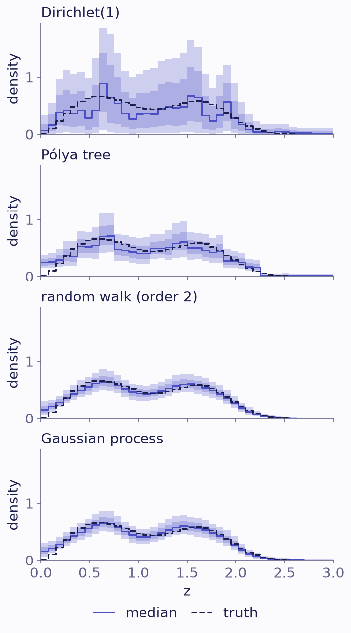
The population posterior (median, 68% and 95% bands) of the same 400 objects under four priors. The truth is dashed.

• The Dirichlet prior Dirichlet(1) adds one pseudo-count to each of the 40 bins: 40 in all, against 400 objects. That raises the fractions in the tails. The bulk is noisy, because mass moves freely between neighbouring bins.

• The Pólya tree shares information between neighbouring bins through its tree of halvings. It is a conjugate prior, so the Gibbs sampler also applies.

• The random walk and the Gaussian process are smoothness priors. They put a prior on the shape of \(\log\rho\) and infer how smooth it is. They give the narrowest bands and still cover the truth.

Dirichlet.reference() sets the concentration \(\alpha_k=1/K\), where \(K=40\) is the number of bins. That is a single pseudo-count in all, which suits many bins with few objects. The engines guide says which sampler handles it best.

Learning the smoothness

binference samples the smoothness hyperparameters \(\theta\) along with the population. Their posteriors show how much structure the data support:

gp = fits["Gaussian process"]
hyper = gp.info["hyperparameters"]
fig, axes = plt.subplots(2, 1)
fig.set_figheight(4.5)
for ax, (name, draws) in zip(axes, hyper.items()):
    ax.hist(draws.ravel(), bins=40, color="C0", alpha=0.8)
    ax.set(xlabel=name, ylabel="draws")
print({k: np.quantile(v, [0.16, 0.5, 0.84]).round(2) for k, v in hyper.items()})

{'amplitude': array([1.6 , 2.24, 3.21]), 'length_scale': array([0.7 , 1.01, 1.46])}

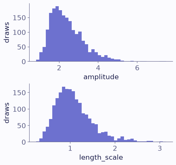
Posterior draws of the Gaussian-process prior’s amplitude (top) and length scale (bottom).

To fix a hyperparameter, pass a number, as in LogisticGP(length_scale=0.3). To change its prior, pass a hyperprior, as in LogisticRandomWalk(scale=priors.HalfNormal(0.2)).

Choosing a prior with held-out data

Which prior describes the population best is partly a scientific choice. Predictive performance is an objective guide. Fit each prior to 300 objects, and score the other 100 with the log predictive density:

train, test = lk[:300], lk[300:]
scores = {}
for name, prior in candidates.items():
    with warnings.catch_warnings():
        warnings.simplefilter("ignore")      # short runs, for speed: two chains of 200
        res = binference.infer(train, prior, rng=2, n_chains=2, n_samples=200, n_warmup=200)
    scores[name] = res.log_predictive(test).sum()
best = max(scores.values())
for name, s in sorted(scores.items(), key=lambda kv: -kv[1]):
    print(f"{name:28s} {s - best:7.1f}")

random walk (order 2)            0.0
Gaussian process                -0.1
Dirichlet(1)                    -2.2
Pólya tree                      -2.2

Higher is better, and the best prior scores zero. Here the two smoothness priors score above the other two. A difference of a few units on 100 objects is suggestive, not decisive. For a more careful comparison, cross-validate over several folds, for example with PopulationEstimator and its score method.

A prior centred on a reference

Outside information, such as a reference sample or a reference distribution, can enter the prior (priors guide). Here a reference distribution is the mean \(\mu\) of a Gaussian-process prior, LogisticGP(mean=np.log(ref)), fitted with NUTS. The reference is deliberately wrong:

ref = binference.simulate.population(bins, "gaussian")   # a deliberately wrong reference
centred = binference.infer(lk, priors.LogisticGP(mean=np.log(ref)), method="nuts", rng=1,
                           n_samples=300, n_warmup=300, n_jobs=-1)
fig, ax = plt.subplots()
centred.plot(ax=ax, truth=mock.truth.rho, label="median")
ax.step(bins.edges[0], np.append(ref, ref[-1]) / bins.volumes[0], where="post",
        color="0.45", lw=1.2, label="reference")
ax.legend(ncol=2, loc="lower left", bbox_to_anchor=(0, 1))
ax.set_xlabel("z");

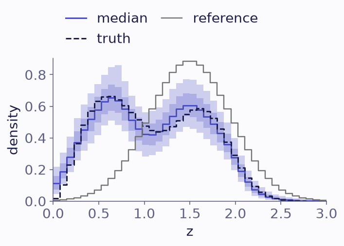
The population posterior under a Gaussian-process prior centred on a reference shape (grey) that is deliberately wrong. The truth is dashed.

The posterior follows the data where they are informative. It stays close to the reference only where they are not.

What to take away

• With sparse data, a smoothness prior gives narrower bands than a Dirichlet prior and still covers the truth here.

• Smoothness hyperparameters are inferred; fix them or change their hyperprior if you know better.

• The log predictive density of held-out objects compares priors on the data. The priors guide lists every prior.