Tutorials / Mixed-stock analysis

Mixed-stock analysis

A fishery catches salmon from several spawning populations, or stocks, that mix at sea. Managers need the stock proportions of the catch, so that weak stocks are not overharvested. Each fish is genotyped. A baseline of fish sampled on the spawning grounds, whose stock is known, gives the allele frequencies of every stock. A fish’s genotype then has a likelihood under each stock. The stock proportions of the catch are population fractions \(\rho_k\) over categorical bins, so this is binference’s model. Any table of likelihoods, one row per object and one column per category, enters the same way. The same analysis estimates the breeding origins of migrating birds and the rookeries of foraging sea turtles.

import matplotlib.pyplot as plt
import numpy as np

import binference

rng = np.random.default_rng(10)

A simulated baseline and mixture

Five stocks, A to E, are typed at 60 loci with two alleles each (SNPs). Their allele frequencies are drawn around a common ancestral frequency, with differentiation \(F_{\rm ST}=0.05\). Stock B is a sister of stock A: its frequencies are drawn around A’s with \(F_{\rm ST}=0.01\), so the two are hard to tell apart. The baseline has 100 fish per stock. The mixture has 1000 fish, most from A and few from B.

stocks = ["A", "B", "C", "D", "E"]
K, n_loci = 5, 60

def drift(p, fst):
    """Allele frequencies of a population descended from frequencies p."""
    c = (1 - fst) / fst
    return np.clip(rng.beta(p * c, (1 - p) * c), 1e-3, 1 - 1e-3)

ancestral = rng.beta(2, 2, n_loci)
freq = np.array([drift(ancestral, 0.05) for _ in range(K)])
freq[1] = drift(freq[0], 0.01)                        # B is a sister stock of A

n_base = 100
baseline = [rng.binomial(2, freq[k], size=(n_base, n_loci)) for k in range(K)]
rho_true = np.array([0.55, 0.05, 0.25, 0.10, 0.05])
origin = rng.choice(K, 1000, p=rho_true)
mixture = rng.binomial(2, freq[origin])               # allele counts, 0 to 2 per locus
print("realised stock shares of this sample:", (np.bincount(origin, minlength=K) / origin.size).round(3))

realised stock shares of this sample: [0.535 0.048 0.283 0.092 0.042]

Genotype likelihoods

The likelihood of a genotype under stock \(k\) assumes Hardy–Weinberg proportions and independent loci. It uses the allele frequencies of stock \(k\) estimated from the baseline, with half a pseudo-allele added on each side. The binomial coefficients are the same for every stock and drop out. from_table takes the table of log-likelihoods as it is:

counts = np.array([b.sum(axis=0) for b in baseline])  # allele counts per stock and locus

def log_likelihood(genotypes, allele_counts, n_fish):
    p = (allele_counts + 0.5) / (2 * n_fish + 1)
    return genotypes @ np.log(p).T + (2 - genotypes) @ np.log1p(-p).T

loglik = log_likelihood(mixture, counts, n_base)      # (fish, stocks)
bins = binference.Bins.categories(stocks)
lk = binference.Likelihoods.from_table(loglik, bins, kind="likelihood", log=True)
fit = binference.infer(lk, rng=1)
print(fit.info["auto_method"], "-", fit.info["auto_reason"])

gibbs - conjugate prior, missing information 0.70

“Classify and count” assigns each fish to its most likely stock and counts the assignments. It is biased: misassigned fish move from abundant stocks to rare ones, so the counts lie closer to equal proportions than the truth does.

assigned = loglik.argmax(axis=1)
cc = np.bincount(assigned, minlength=K) / assigned.size
lo, hi = fit.interval(0.9)
print("stock  truth  classify-and-count  binference (90% interval)")
for k, s in enumerate(stocks):
    print(f"  {s}    {rho_true[k]:.2f}   {cc[k]:.3f}               "
          f"{fit.mean[k]:.3f} [{lo[k]:.3f}, {hi[k]:.3f}]")

stock  truth  classify-and-count  binference (90% interval)
  A    0.55   0.320               0.411 [0.374, 0.449]
  B    0.05   0.232               0.166 [0.134, 0.201]
  C    0.25   0.277               0.288 [0.264, 0.313]
  D    0.10   0.103               0.093 [0.077, 0.110]
  E    0.05   0.068               0.041 [0.029, 0.054]

The fit reduces the bias of counting, but its intervals for the sister stocks A and B are narrow and miss the truth. The likelihoods treat the baseline allele frequencies as exact. With 100 fish per stock they are not. Their errors matter most for A and B, because only small differences in frequency separate those two stocks.

Carrying the baseline’s uncertainty

binference cannot infer allele frequencies, but it can infer a confusion matrix together with the proportions. Assign every baseline fish with frequencies estimated from the other baseline fish, so that no fish helps to classify itself. Then tally the assigned stock against the known stock with from_labelled(). Each column of the tally gets a Dirichlet posterior, inferred with the proportions. The mixture fish enter only through their assigned stock (from_binned()). This is the route of “scores and a labelled set” in Classifier outputs: class fractions under label shift, with the baseline as the labelled set.

labels, predicted = [], []
for k in range(K):
    for g in baseline[k]:
        c, n = counts.copy(), np.full((K, 1), float(n_base))
        c[k] -= g
        n[k] -= 1
        predicted.append(int(log_likelihood(g[None], c, n).argmax()))
        labels.append(k)
labels, predicted = np.array(labels), np.array(predicted)
print(f"baseline self-assignment rate: {np.mean(labels == predicted):.3f}")

response = binference.Response.from_labelled(
    np.array(stocks)[predicted], np.array(stocks)[labels],
    measured_bins=bins, classes=stocks,
)
print("confusion matrix, P(assigned row | true column):")
print(response.matrix.round(2))

baseline self-assignment rate: 0.794
confusion matrix, P(assigned row | true column):
[[0.58 0.31 0.   0.04 0.05]
 [0.37 0.66 0.01 0.02 0.04]
 [0.   0.   0.98 0.01 0.05]
 [0.01 0.02 0.   0.92 0.03]
 [0.04 0.01 0.01 0.01 0.83]]

A and B are confused with each other far more often than any other pair. The fit infers the 25 cells of the confusion matrix with the proportions. Gibbs mixes slowly for this joint model, because the classes overlap this much, so method="auto" chooses NUTS:

lk_c = binference.Likelihoods.from_binned(response, values=np.array(stocks)[assigned])
fit_c = binference.infer(lk_c, rng=1)
print(fit_c.info["auto_method"], "-", fit_c.info["auto_reason"])
d = fit_c.diagnostics
print(f"max R-hat {d['rhat'].max():.3f}, min bulk ESS {d['ess_bulk'].min():.0f}, "
      f"divergent {d['n_divergent']}")

nuts - Gibbs mixed too slowly; the Laplace importance check failed
max R-hat 1.004, min bulk ESS 969, divergent 0

from binference.plotting import SAMPLE_COLOR
fig, ax = plt.subplots()
fig.set_figheight(3.8)
pos = np.arange(K)
for dx, res, name, color, marker in [(-0.14, fit, "baseline fixed", "C0", "o"),
                                     (0.14, fit_c, "matrix inferred", "C1", "^")]:
    lo, hi = res.interval(0.9)
    ax.errorbar(pos + dx, res.mean, yerr=[res.mean - lo, hi - res.mean], fmt=marker,
                color=color, ms=8, capsize=3, label=name)
ax.plot(pos, cc, "s", color=SAMPLE_COLOR, ms=8, label="counting")
ax.plot(pos, rho_true, "_", color="k", ms=26, mew=2, label="truth")
ax.set(xticks=pos, xticklabels=stocks, xlabel="stock", ylabel="proportion")
ax.legend(ncol=2, loc="lower left", bbox_to_anchor=(0, 1));

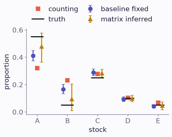
Stock proportions with 90% intervals. Circles, baseline fixed. Triangles, confusion matrix inferred. Squares, classify and count. Bars, truth.

lo_c, hi_c = fit_c.interval(0.9)
for k, s in enumerate(stocks):
    print(f"  {s}: {fit_c.mean[k]:.3f} [{lo_c[k]:.3f}, {hi_c[k]:.3f}]   truth {rho_true[k]:.2f}")

  A: 0.478 [0.363, 0.577]   truth 0.55
  B: 0.095 [0.010, 0.204]   truth 0.05
  C: 0.282 [0.253, 0.311]   truth 0.25
  D: 0.099 [0.075, 0.121]   truth 0.10
  E: 0.046 [0.015, 0.073]   truth 0.05

With the confusion matrix inferred, the intervals for A and B widen, because the baseline separates them weakly, and they cover the truth. Stocks C and D, which the baseline separates well, keep narrow intervals. The cost is lost information: each mixture fish contributes only its assigned stock, not its full likelihood.

What to take away

• Stock proportions are a population over categorical bins (Bins.categories). Any table of likelihoods enters through Likelihoods.from_table(..., kind="likelihood"), here with log=True.

• Likelihoods from estimated baseline frequencies are treated as exact, so intervals can be too narrow for stocks that the baseline separates poorly.

• A confusion matrix tallied from the baseline (Response.from_labelled) carries that uncertainty, at the cost of using only each fish’s assigned stock.